Understanding Few-Shot Multi-Task Representation Learning Theory

25 Mar 2022 | multi-task-learning few-shot-learning learning-theory Bouniot, Quentin; Redko, Ievgen

Learning something new in real life does not necessarily mean going through a lot of examples in order to capture the essence of it. Even though it is said that it takes 10,000 hours to master a new skill, it is also true that it only takes 20 hours to learn it. This is particularly the case for classification tasks, for which we are often capable of differentiating between two distinct objects after having seen only a few examples of them. This idea has found its application in machine learning in a more general few-shot learning paradigm that wants to mimic the human capability to quickly learn how to solve a new problem.

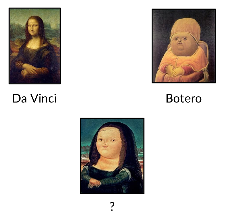
Credits to F. Botero and L. Da Vinci

As an illustrative example, let’s take a look at these paintings from Leonardo Da Vinci and Fernando Botero. It is quite obvious that one would easily guess and recognize the painter who did the painting below after having seen just one example of each painter’s styles. This is a prime example of datum science a.k.a one-shot learning.

Who called it “one-shot learning” and not “datum science”?

— Daniel Lowd (@dlowd) October 27, 2021

Recently, researchers have turned to Meta-Learning for solving the few-shot learning problem. The general idea behind Meta-Learning is to learn how to learn a new task quickly, i.e, with few examples. A common approach to this is to construct and make the models learn on a lot of such small tasks. Meta-learned models currently achieve relatively good performance on few-data tasks, but there is still a high variance in the results depending on the inner-hardness of the task. One could say that these models are sort of jack of all trades … but master of none.

At the same time, learning multiple tasks simultaneously is also the key point of a conceptually similar, yet much better understood and studied Multi-Task Representation Learning paradigm. As meta-learning still suffers from a lack of theoretical understanding for its success in few-shot tasks, an intuitively appealing approach would be to bridge the gap between it and multi-task learning to better understand the former using the results established for the latter. Before this, we need to improve the theory behind multi-task learning to explain how to use all source data coming from many small tasks. In particular, a recent ICLR 2021 paper¹ proved novel learning bounds demonstrating its success in the few-shot setting. Below, we dive into this work and go beyond it by establishing the connections that allow to better understand the inner workings of meta-learning algorithms as well.

Multi-Task Representation Learning

Notations

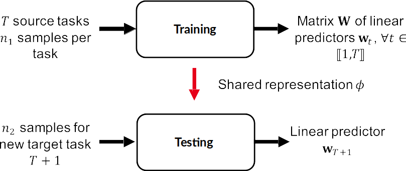
First, let’s review the working setup used in their paper. In Multi-Task Representation Learning (MTR) – a setting where a common shared representation is learned for a set of tasks – we have $T$ source tasks with $n_1$ examples each. For each task $t \in [1, \dots, T]$, the $n_1$ data are sampled i.i.d from a distribution $\mu_t$. During the training phase, we learn a linear predictor $w_i$ for each task and then group them all in a matrix $W$. Throughout training, a common representation $\phi \in \Phi$ is learned, that we use afterwards for a novel target task $T+1$ with $n_2$ examples sampled from $\mu_{T+1}$. Using this common representation, we learn a novel predictor $w_{T+1}$ for the target task.

Multi-Task Learning Bounds

While empirically such an approach is known to work well, one may ask whether there exists a theoretical explanation for such success? The latter justification usually takes the form of inequalities, also known as learning bounds, that seek to upper-bound the error in the target domain by other quantities involved in the solved problem. Below, we quickly review such results for multi-task learning, that backup the success of MTR in practice.

Historical Review

The main idea of Multi-Task Representation Learning is that all the tasks considered are related by an underlying common representation, where the latter is learned by jointly training on these tasks. In the seminal work on multi-task representation learning theory, Baxter ² defined what they call environments of tasks. This means that the generation of the tasks is subject to a common underlying law $\nu$. They assumed that there exists environments of related tasks, and that the training and testing tasks come from the same environment:

Assumption 1²³:

\[\forall t \in [1, \dots, T+1], \mu_t \sim \nu\]

One may think of an environment as of a dataset generator that outputs a set of tasks to learn on. In a more recent work Maurer et al. ³ obtained a bound for MTR in the form of $O(\frac{1}{\sqrt{n_1}} + \frac{1}{\sqrt{T}})$, where $n_1$ is the number of training data available in each training task, and $T$ is the number of tasks seen during the training phase. One should note that this bound does not give us insight for the few-shot setting as we have no information coming from the number of test samples, and according to it both the number of seen training samples and the number of tasks should tend to infinity. Maurer et al. even provide an example for which a $\frac{1}{\sqrt{T}}$ rate was unavoidable and could not be improved on.

The New Bounds

To address the latter drawback, Du et al. provided learning bounds specifically for few-shot learning setting within MTR framework. The intuition behind their work is to say that the success in few-shot learning should rely on all of the source data given by $n_1*T$ such that considering a lot (large $T$) small tasks (small $n_1$) should be sufficient, from the theoretical point of view, to learn well. But to do so, they need to introduce additional assumptions on the relations between the tasks, as opposed to only the i.i.d assumption used above in the works of Baxter and Maurer et al. The paper of Du et al. considers MTR in different flavours depending on how exactly the common representation is learned and we review those settings and the assumptions associated to them below.

Review of assumptions

Readers familiar with the statistical learning literature should brace themselves at this point as quite often the statements of theorems are much more complicated and hard to understand than the final results themselves. The paper we are presenting is not an exception from this rule but fear not, our dear readers! Bear with us as we go through the dark dungeons of assumptions made throughout their paper and try our best in explaining them using simple examples. Don’t let yourself be daunted by all of these assumptions ! Fortunately, they are not required simultaneously in the different settings considered in the paper and detailed below.

Let’s proceed with these two for starters.

Assumption 2.1¹:

\[\text{Sub-Gaussian input.}\]

Assumption 2.2¹:

\[\text{Normalized linear predictors.}\]

Both of these assumptions are common in statistical learning. The first one requires the tails of data generating distributions to be well-behaved. In simple words, if my distribution generates images of popular musicians of the last decade, then I should not see many weird-looking singing robots with a pigtails instead of the nose that went viral on Youtube in my learning sample. There may be some, but really few!

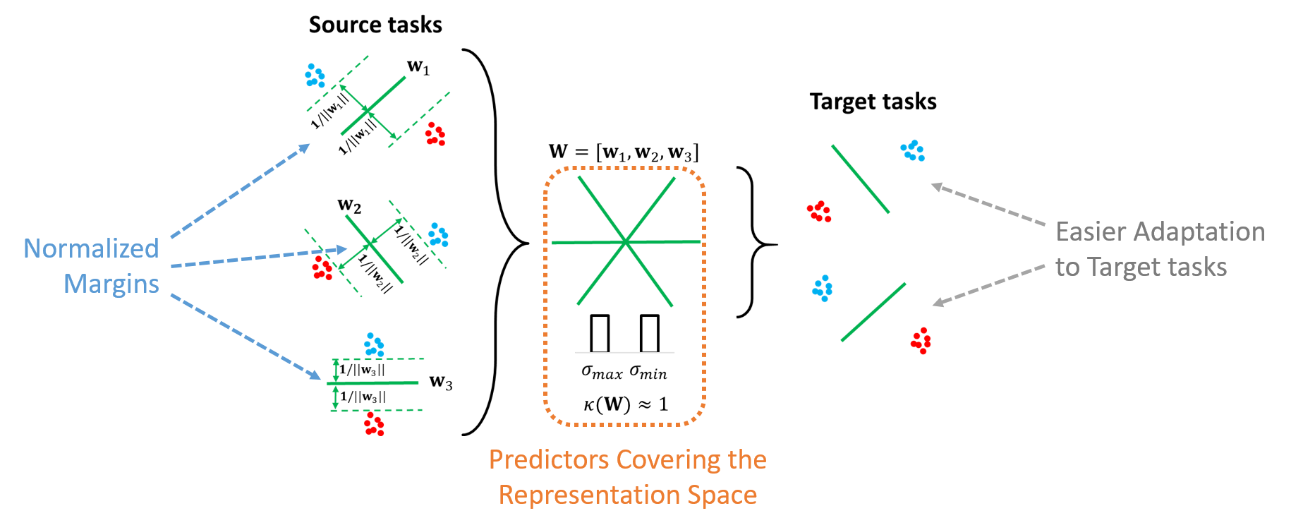
The second one is to ensure that the classification margin of the optimal predictors stays constant throughout the training phase. In practice, this means that the norm of the predictors must not increase with the number of training tasks seen as if we were to make sure that all tasks are treated with an equal level of respect. This assumption is not explicitly stated in the paper, but it is used multiple times in key developments and to better understand the other assumptions. It also seems to be an important setting discussed in the following papers that we mention below.

Assumption 2.3¹:

\[\text{Diversity of the source tasks.}\]

Assumption 2.4¹:

\[\text{Target task evenly represented or coherent with the source tasks.}\]

Assumption 2.3 is related to the diversity of the source tasks seen during training and requires from optimal source predictors to evenly cover the representation space. Informally, if I learn to recognize musicians by only comparing them either to Billie Eilish or to Elvis Presley, then I should not be expected to be good at telling the difference between Eminem and Nina Simone at test time. More formally, this means that the condition number of the matrix of the optimal predictors must not increase when the number of tasks seen increases: I should not concentrate too much on some tasks but neglecting others. As a reminder for people who missed on some linear algebra basics, the condition number is defined as the ratio between the largest and the smallest singular values.

Assumption 2.4 makes sure that the target task does not align particularly with some directions of the representation space. It is similar to Assumption 2.3 but from the target task’s point of view. Getting back to the musicians example, that would mean that if I am learning on data from all music genres (source tasks), I may not be super-efficient in classifying Kawai core (target tasks and yes, that’s a real thing!) musicians from early 90s: the latter are too specific and fine-grained for the representation space that I am learning.

Assumption 2.5¹:

\[\text{Covariance dominance of the source tasks.}\]

Assumption 2.5 takes into account the similarity between the source tasks and the test tasks, by considering that the covariance in the data of the former dominates the covariance in the data of the latter by a factor $c$. As we will see in the next section, the latter factor appears in the bounds and affects directly the success of few-shot learning. Want another music example? It is hard to come up with one on this case but maybe this will do: consider that the variety of different musicians that I learned on should be at least on par with the variety of musicians for which I am supposed to make predictions afterwards.

Assumption 2.6¹:

\[\text{Input data from all tasks follow the same distribution.}\]

This assumption may seem too restrictive at first sight but it actually only means that our data comes from the same distribution without putting any constraints on the labels associated to it. In our previous example, it means that the common distribution are just all the musicians from a certain decade and our small tasks can be learning different genres from it.

Assumption 2.7¹:

\[\text{Point-wise and uniform concentration of covariance.}\]

The concentrations of covariances assumptions ensure that even though we are working in a few-shot learning setting, there is enough data for the empirical covariance to be close to the true covariance. This roughly means that we want to make sure that our few data points are representative of the covariance of the data generating distribution.

Now, the worst is behind us and we can enjoy the insightful learning bounds for few-shot learning in MTR framework without all the cumbersome hypotheses used to derive them.

The different settings

Now let’s see what bounds we can obtain for the different settings of interest. The latter cover:

1. Linear low-dimensional representations = multiply the input data with some matrix projecting it to a low-dimensional space.
2. General low-dimensional representations = learning a low-dimensional embedding with non-linear functions.
3. Linear high-dimensional representations = learning a linear map (a matrix) without any constraints on its size.

The first case gives the most explicit expression of the learning bounds that highlights the importance of the different factors involved in it. It can be formulated in a concise form as follows:

\[\substack{\Large{\text{Linear low-dimensional}}\\\Large{\text{representation function}}}\quad + \quad \substack{\Large{\text{Assumptions}}\\\Large{\text{2.1-5}}}\quad = \quad O\Big(\frac{dk}{c n_1 T} + \frac{k}{n_2}\Big)\]

One can note that the factor of covariance dominance $c$ as defined in Assumption 2.5 appears in the bound as well as the dimensionality of the input space $d$, that of the embedding $k \ll d$ and the sizes of source and target samples $n_1$ and $n_2$.

Let’s now present the second case where a non-linear function is used to project the input data to a low-dimensional space. In this case, the bound can be summarized as follows:

\[\substack{\Large{\text{Non-linear low-dimensional}}\\\Large{\text{representation function}}}\quad + \quad \substack{\Large{\text{Assumptions}}\\\Large{\text{2.1-4, 2.6-7}}}\quad = \quad O\Big(\frac{\mathcal{C}(\Phi)}{n_1 T} + \frac{k}{n_2}\Big)\]

An important difference of this bound when compared to the linear case is that it also depends on $\mathcal{C}(\Phi)$, the complexity of the class of representation function $\Phi$ considered. This is intuitive as in order to learn more complex embeddings one may need access to more data or to seeing more different tasks. In the general case, this complexity can be computed as the Gaussian width of the space spanned by the features obtained from the input data.

In the third case, when the dimensionality constraint is removed, Du et al. obtain the following result:

\[\substack{\Large{\text{High-dimensional linear}}\\\Large{\text{representation function}}}\quad + \quad \substack{\Large{\text{Assumptions}}\\\Large{\text{2.1-2, 2.4, 2.6}}}\quad = \quad O\Big(\frac{\bar{R}\sqrt{\text{Tr}(\Sigma)}}{\sqrt{n_1 T}} + \frac{\bar{R} \sqrt{\| \Sigma\|_2}}{\sqrt{n_2}}\Big)\]

This bound depends on the covariance matrix of the input data $\Sigma$ and $\bar{R}$ a normalized nuclear norm over the linear predictors. The authors also extend this result to the case of two-layer ReLU neural networks using an additional assumption on the labeling of the source tasks (Assumption 7.1 in the original paper).

Insights

It’s all fine and nice to present the learning bounds in different cases but what are exactly the insights that we can get from them? Below, we formulate two key findings derived from the discussed work.

1. All source data is useful for learning the target task!

   This is the key achievement of this work compared to other studies as it tells us that under some assumptions between the tasks we can expect to perform well on the target task after having seen many small source tasks just as we can do it in practice. Once again, this is different from saying that one has to provide both a huge number of tasks and data samples of big size to achieve the same goal as suggested by earlier works on the subject.

2. The assumptions reveal the a priori success of few-shot learning and give practical guidance!

   This insight is even more important as it tells us when one can learn efficiently in few-shot setting. On the one hand, it tells us that there are some a priori assumptions required for the success in few-shot learning setting. Those are Assumptions 2.1, 2.4, 2.6 and 2.7. We cannot do much about those except for crossing fingers and hoping that they are satisfied.

   On the other hand, the second group of assumptions includes Assumption 2.2 and 2.3. These assumptions are of primary interest as they involve the matrix of predictors of the source tasks that we are learning from. Even though they are referring to the optimal quantities, for which we have no information, it can guide us to learn more efficiently, as we will see further below. It is worth noting that in a concurrent work to Du et al., Tripuraneni et al. ⁴ achieved similar learning bounds in the linear case, using only an equivalent of Assumptions 2.1, 2.2 and 2.3. This emphasizes the intuition that normalized predictors (Assumption 2.2) and diverse source tasks (Assumption 2.3) seem to be important features for multi-task learning.

   Finally, we note that Assumption 2.5 related to the covariance dominance can be seen as being at the intersection between the two groups. Indeed, at the first sight it is related to the population covariance and thus to the data generating process that is supposed to be fixed. However, we can think about a pre-processing step that precedes the training step of the algorithm that transforms the source and target tasks’ data so that their sample covariance matrices satisfy it. Applying this constraint in practice may present an interesting open avenue for future works.

Beyond multi-task learning: Meta-learning

The attentive reader may feel cheated at this point as we haven’t said anything about the link between multi-task learning and meta-learning up until now despite it being advertised in our introduction section. We will now do justice to it by first presenting the meta-learning framework and by mentioning another recent works that connect it nicely to multi-task representation learning.

Meta-Learning 101

The goal of Meta-Learning is to learn a meta-learner on a large number of tasks: the primary goal is thus not to learn a classifier as in supervised learning but a model that can be adapted to new tasks efficiently. In practice, the model is often a deep neural network that embeds the data in a common representation space. The latter process is repeated over a distribution of tasks where a given task is a sub-problem of the problem that we want to solve. For instance, in the case of image classification, a task is a sub-problem of classification for a particular choice of classes. For each of these tasks, the meta-learner trains a learner: we can think of them as of predictors trained specifically for each task with, for instance, SVM, ridge regression or gradient descent. Finally, the meta-learner is evaluated on novel tasks that were not seen during meta-training.

As mentioned above, meta-learning is a popular choice nowadays when dealing with few-shot learning problems. In this case, the task that we construct for the meta-learner consists of only a handful of data points. This way, the meta-learner learns to learn with few data, and, when faced with a novel task for which few data is available, it is capable of quickly adapting and producing a learner to solve it.

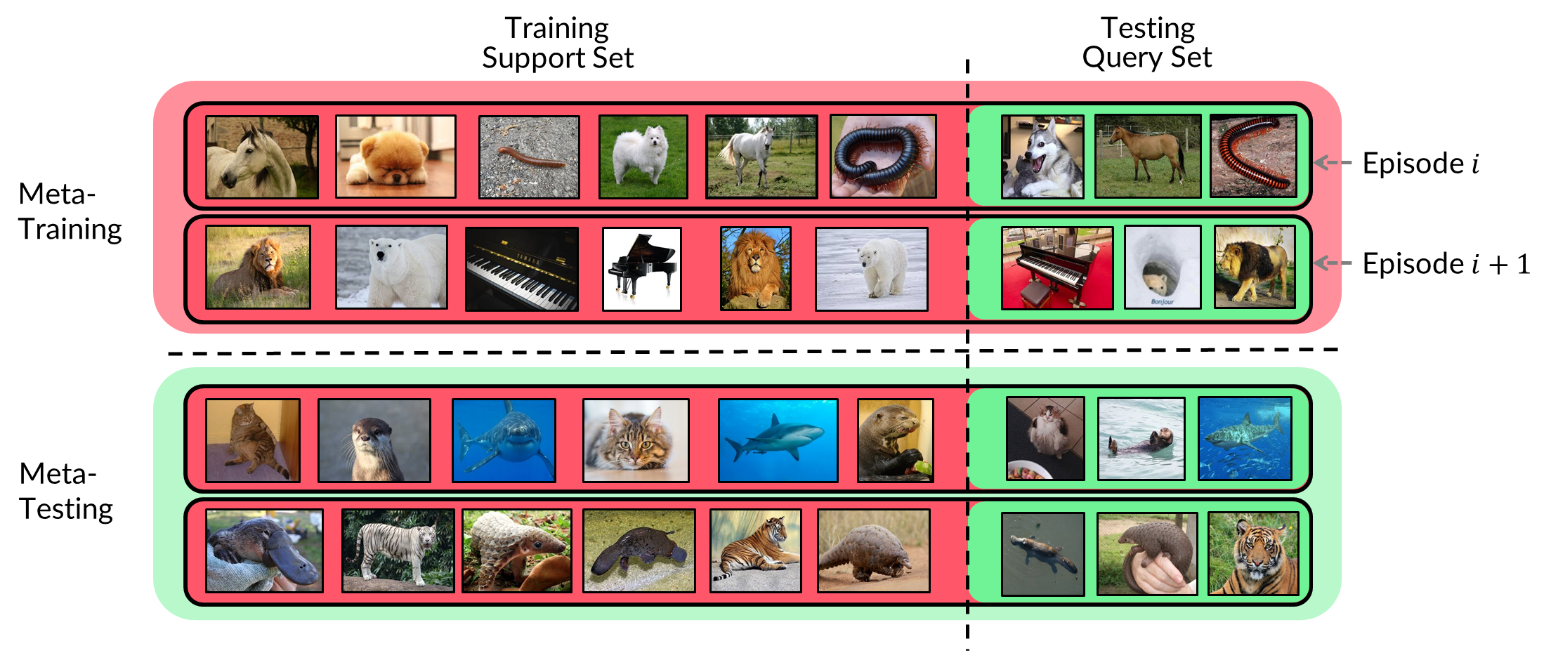
Credits to oneweirdkerneltrick

How do we meta-learn in practice? To do so, we construct episodes. An episode is an instance of a sub-problem of the problem we want to solve. For example, for a specific sub-problem of classification of dogs and cats, it will contain a training and a testing set of images of dogs of cats. In the episode, the training set is called support set, and the testing set is called query set. Then, these episodes are separated into meta-training episodes and meta-testing episodes. The meta-learner is trained on the meta-training episodes and evaluated on the meta-testing episodes. In the case of classification problems, an N-way k-shot episode is an instance with N different classes and k images per class.

Link between multi-task and meta-learning

At this point you’ve probably noticed that meta- and multi-task learning have lots in common but they also bear a crucial difference that do not allow to treat them as strictly the same. Let’s talk about both similarities and distinctions below.

1. Similarities

   The most important similarity between the two frameworks is that they both learn a common representation from a set of tasks in order for it to be efficiently applied to solve a new previously unseen task. In principle, we can see the training phase in the MTR learning setup as meta-training phase of meta-learning, and, similarly, for the testing task and the meta-testing tasks on which we evaluate our meta-learner.

2. Differences

   The most important difference between the two lies in the way they are implemented in practice: multi-task algorithms learn source tasks simultaneously while meta-learning does that sequentially by learning on the support set and then the query set of the constructed episodes. More formally, it means that multi-task learning methods are solved by a simple joint optimization, whereas meta-learning algorithms use a bi-level optimization procedure.

One may wonder if there is a way to alleviate the difference between the two and to leverage on their similarity to gain insights into meta-learning? To answer this question, we should first note that some meta-learning algorithms have independent parameters for each level of the optimization procedure. For example, the popular Prototypical Networks, introduced by Snell et al. ⁵, construct prototypes from the task training data, and optimize the representation with the task testing data. Similarly, the recent ANIL, from Raghu et al. ⁶, is a modification of the popular MAML, introduced by Finn et al. ⁷, that separates the learning of the linear predictors on the support set (inner-loop or adaptation phase) from the learning of the encoder on the query set (outer-loop).

In these specific but recurring cases, Wang et al. ⁸ showed that the episodic framework converges to a solution of the bi-level optimization problem that is close to solution of the joint multi-task learning problem. Their main result can be stated in the case of ANIL and a MTR learning algorithm as follows:

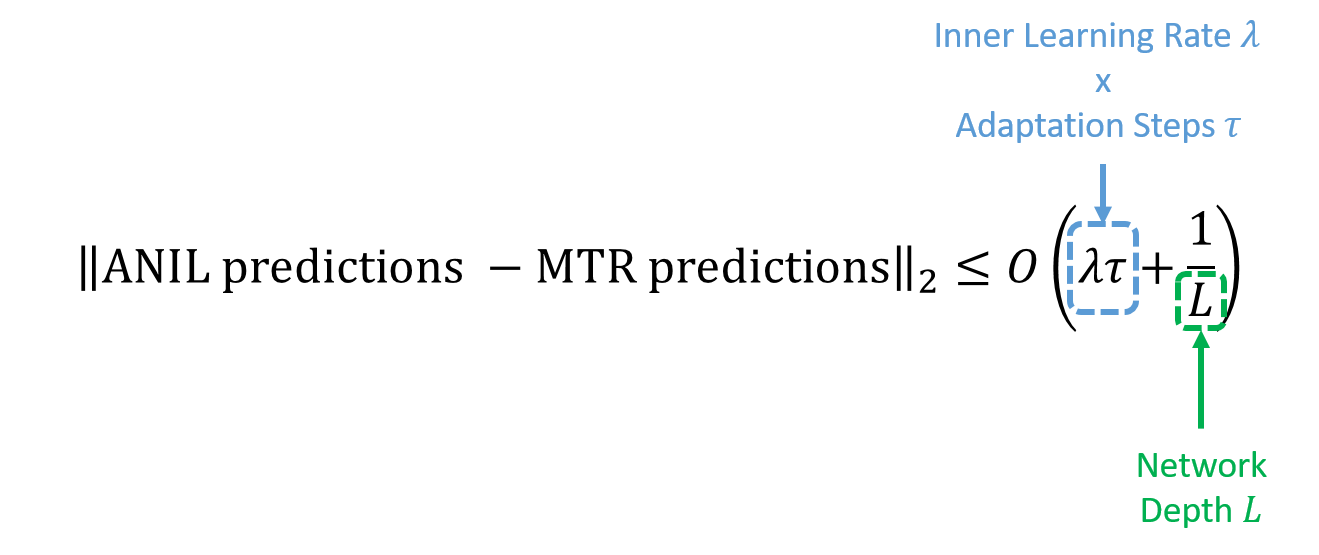
As we have typically in practice a low inner-loop learning rate and few adaptation steps as well as a deep neural network, both of the terms bounding the differences in the predictions are small. It means that the learned representation obtained in both cases is negligibly similar and thus the results from the work of Du et al. directly apply in this case. To confirm this, Bouniot et al. ⁹ made an empirical analysis of popular meta-learning algorithms in light of the novel assumptions proposed by Du et al.

Adapted from Bouniot et al.

They showed that satisfying or not these two assumptions can reveal striking differences in the behavior of these algorithms. Their results highlight the importance of the assumptions 2.2 and 2.3 for an efficient few-shot learning in practice.

Conclusion

The theoretically involved paper of S. Du, W. Hu, S. Kakade, J. Lee and Q. Lei that recently appeared in ICLR 2021, studies multi-task representation learning in the few-shot setting and demonstrates its theoretical success. The authors show that with the right assumptions, we can achieve learning bounds with a coupling between the number of tasks seen during training and the number of training data for each task, implying that we can reduce one or the other to reduce the target risk. Their results have already started to make impact in the few-shot learning community, with some preliminary results showing that an in-depth analysis of the assumptions used could lead us to more efficient algorithms for few-shot learning and to bridging the gap between the multi-task learning theory and the practice of meta-learning.

References