An Understanding of Learning from Demonstrations for Neural Text Generation

25 Mar 2022 | natural-language-generation reinforcement-learning generative-models Kantharaju, Pavan, Smart Information Flow Technologies; Sankar, Aiswarya, Independent

In this blog post, we will go over the ICLR 2021 paper titled Text Generation by Learning from Demonstration. This paper introduces a learning method based on offline, off-policy reinforcement learning (RL) which addresses two key limitations of a training objective used in neural text generation models: Maximum Likelihood Estimate (MLE).

Goal of this blog post: Our main goal with this blog post is to provide researchers and practitioners in both NLP and RL with (1) a better understanding of algorithm presented in this paper (GOLD), and (2) an understanding of how RL is used for text generation.

The Problem with Text Generation via MLE

Text-Gen-Diagram

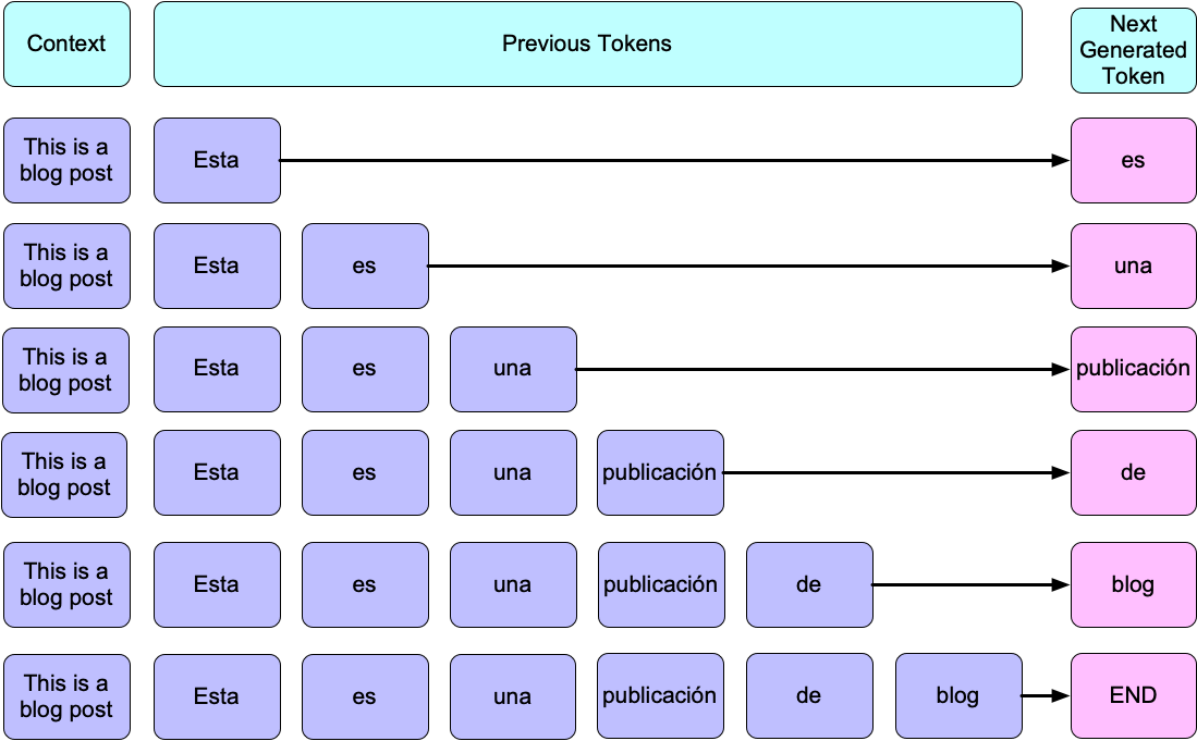
The standard method for language generation relies on autoregressive models learned using an MLE objective function. Autoregressive models generate text sequentially by predicting the next token to generate based on a history (i.e., previously-generated tokens). The above image provides an example of how an autoregressive model generates a translation of the English text “This is a blog post” to its Spanish counterpart: “Esta es una publicaión de blog.”

At a high level, the MLE objective function for text generation aims at maximizing the probability of a token given previous text and some context. In the above figure for example, the MLE objective would teach a generation model to assign high probability to “publicaión” given the context “This is a blog post” and history “Esta es una”.

While the MLE objective has seen incredible success, it suffers from two unfortunate problems:

Exposure Bias - The history used to predict the next token differs between training and evaluation. During evaluation, this is text generated by the model (i.e., previously-predicted text is used as input to predict new tokens). However, during training, this is the gold standard text found in the training dataset. This is rather problematic because the training process draws tokens from the training data’s token distribution whereas evaluation draws tokens from the model’s token distribution (Ranzato et al., 2016). Thus, one incorrect error during token prediction and the model (1) cascade errors for subsequent predictions and (2) produce text that is unlikely under the gold standard’s distribution.
Training + Evaluation Metric Mismatch: We train generation models using MLE, but we evaluate them using metrics such as F1-score, BLEU (Papineni et al., 2002), or ROGUE (Lin, 2004). This means that we are not optimizing our model to generate text that addresses these metrics.

The paper we describe in this blog post introduces a method called Generation by Off-policy Learning from Demonstrations (GOLD) that utilizes RL methods to fine-tune a text-generation model trained using MLE. GOLD addresses the above problems as follows:

Exposure Bias: Similar to MLE training, GOLD trains the model to choose the next token given a context and history comprised of gold standard text. However, GOLD additionally uses importance weighting with the gold standard text as a way to guide the model to learn training samples with high likelihood under the model.
Training + Evaluation Metric Mismatch: GOLD guides the training of a text generation model to construct text with high-quality using a reward signal that approximates an evaluation metric. For generality, this paper uses perceptual quality of text as the evaluation metric (i.e., measure of how likely a human would have generated a text) (Huszar, 2015), (Hashimoto et al., 2019).

We begin by providing some background on the RL concepts that we will see in this blog post and how those concepts relate to MLE.

Background

From the initial $n$-gram language models to the various iterations on Transformer based language models of today, language generation has long formulated itself as essentially a maximum likelihood estimation (MLE) problem. The question we ask when using MLE is: given the history of $n$ words $x_1, \dots, x_i$ from a sentence $x = \langle x_1, \dots, x_n \rangle$, how likely will a generation model predict $x_{i+1}$ next? MLE formalizes this question by computing the probability distribution over the entire vocabulary of next possible words and choosing the word with the highest probability.

Despite its wide adoption for text generation, MLE does have a few limitations. One limitation is that MLE doesn’t allow for any exploration - at each time step the likelihood is maximized and that is selected as the next output. However, the core problem with MLE methods is the discrepancy between the training and evaluation objectives. The training process maximizes the expected likelihood of a training dataset while the evaluation process maximizes the performance over an evaluation metric. In order to address this problem, we can instead reformulate the text generation problem as a Reinforcement Learning (RL) problem. Specifically, RL enables us to focus on maximizing the performance over evaluation metrics or text quality metrics during training in addition to evaluation.

Reinforcement Learning is the branch of machine learning that aims to find an optimal behavior strategy (or policy) for an agent to obtain optimal rewards in an environment. These problems are formulated as an actor taking some action in a state to transition to a new state where it gets a reward for having taken that action. In the context of text generation, a text generation model is the policy being optimized, states are the word sequences of a text generated so far and the source text, actions are represented as choosing a next word, and rewards represent the quality of the next word generated.

The RL framework can be addressed using several different algorithms which can be categorized as falling under the fields of value-based, policy-based or model-based approaches. Value-based RL aims to learn the state or state-action value. Value-based RL is generally adopted through Q-learning where the average expected reward at each state is estimated. Model-based RL aims to learn the model of the world and then plan using the model. The model is updated and re-planned often. Policy-based RL aims to directly learn the stochastic policy function that maps state to action. The agent acts by sampling from the policy. The paper presented in this blog post focuses on a policy-based RL approach called policy gradient.

Policy Gradient

Before diving into how the paper makes use of offline policy gradients to address the shortcomings of MLE, we will first give some background on policy gradient and mention how it relates to MLE. The goal of reinforcement learning can be formalized as finding the policy $\pi$ that maximizes the expected sum of rewards (if the policy is parameterized, then we are finding a parameterized policy $\pi_{\theta}$):

\[J = max_{\pi_{\theta}}~\mathbb{E}_{\tau \sim \pi_{\theta}} \Big[ \sum_{t=0}^{T} \gamma^t R(s_t, a_t) \Big]\]

We will now derive the policy gradient update from this objective function. Let $\tau = \langle s_0, a_0, \dots , s_T, a_T \rangle$ denote a path or a trajectory (i.e., state-action sequence) and the reward function over this path as $R(\tau) = \sum_{t=0}^{T} R(s_t, a_t)$. First, let’s start by taking the gradient with respect to $\theta$:

\[\begin{align*} \nabla_{\theta} J(\theta) & = \nabla_{\theta} \sum_{\tau} P(\tau; \theta) R(\tau) = \sum_{\tau} \nabla_{\theta} P(\tau; \theta) R(\tau) \\ & = \sum_{\tau} \frac{P(\tau; \theta)}{P(\tau; \theta)} \nabla_{\theta} P(\tau; \theta) R(\tau) \\ & = \sum_{\tau} P(\tau; \theta) \frac{\nabla_{\theta} P(\tau; \theta)}{P(\tau; \theta)} R(\tau) \\ & = \sum_{\tau} P(\tau; \theta) \nabla_{\theta}~log P(\tau; \theta) R(\tau) \end{align*}\]

where $P(\tau; \theta) = \prod_{t=0}^{T} P(s_{t+1} | s_t, a_t) \pi_{\theta}(a_t | s_t)$. Now we approximate with the empirical estimate for $M$ sample paths under policy $\pi_{\theta}$.

\[\nabla_{\theta} J(\theta) \approx \frac{1}{M} \sum_{i=1}^{M} \nabla_{\theta}~log P(\tau^i; \theta) R(\tau^i)\]

This equation is valid even when $R$ is discontinuous and you have a discrete set of paths. Now we can calculate the probability of a path, which consists of taking the product of the dynamics model or the probability of transitioning from a state given the current state and the applied action:

\[\begin{align*} \nabla_{\theta} log~P(\tau^i; \theta) & = \nabla_{\theta} log~ \Big[ \prod_{t=0}^{T} P(s_{t+1}^i | s_t^i, a_t^i) \pi_{\theta}(a_t^i | s_t^i) \Big] \\ & = \nabla_{\theta} \Big[ \sum_{t=0}^{T} log~P(s_{t+1}^i | s_t^i, a_t^i) + \sum_{t=0}^{T} log~\pi_{\theta}(a_t^i | s_t^i) \Big] \\ \end{align*}\]

The dynamics model isn’t needed in this case because it doesn’t depend on $\theta$ and thus:

\[\nabla_{\theta} log~P(\tau^i; \theta) = \nabla_{\theta} \sum_{t=0}^{T} log~\pi_{\theta} (a_t^i | s_t^i)\]

This brings us finally to the policy gradient:

\[\nabla_{\theta} J(\theta) = \mathbb{E}_{\tau \sim \pi_{\theta}} \Big[ \sum_{t=0}^{T} log~\pi_{\theta}(a_t|s_t) R(\tau) \Big]\]

Compared to the MLE objective, this is the exact same equation except that the policy gradient update equation includes $R(\tau)$ whereas MLE doesn’t. With policy gradients, the agent is able to explore and thus needs to receive a reward for the action whereas with MLE there is only one possible action to take which is the maximum likelihood with reward 1.

Off-Policy vs On-Policy Learning

Given that we now understand the connection between policy gradient and MLE, we now turn our focus to on-policy learning and, the method that GOLD uses, off-policy learning. On-policy RL samples from the current policy when deciding next actions whereas off-policy RL samples from an another policy. This distinction can be made for value-based, model-based and policy-based RL approaches. For example, within value-based RL, Q-learning is an off-policy approach whereas SARSA (state-action-reward-state-action) is on-policy. This is because Q-learning uses $\epsilon$-greedy as the policy to determine actions which is different from the current learned policy. SARSA instead uses the current policy in order to determine actions. A similar paradigm applies to policy gradient approaches.

If training samples are collected through the policy we try to optimize for, it is called an on-policy algorithm. However, this means that we cannot use training samples from previous training steps, as they were collected with a different version of the policy. This is where off-policy algorithms have an advantage: off-policy algorithms do not require that the training samples are collected with the current policy. Off-policy algorithms have a “behavior policy” that is used to collect training samples to train the “target policy.” Having a behavior policy allows the agent to be more explorative while collecting experience. Furthermore, an off-policy algorithm allows the agent to save and reuse past experience for better sample efficiency.

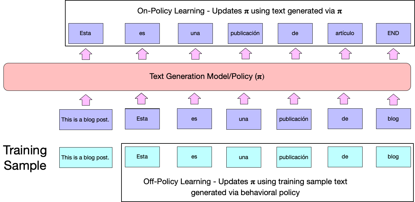
Both off-policy and on-policy approaches have been used for RL-based neural text generation on a variety of tasks including dialogue generation (Li et al., 2016), (Li et al., 2017), (Kandasamy et al., 2017), and machine translation (Ranzato et al., 2016), (Bahdanau et al., 2017). The fundamental difference between on-policy and off-policy methods for RL-based neural text generation is the origin of the text used to update the policy. In the case of off-policy learning, this text is from a training dataset or set of demonstrations generated by a separate behavioral policy rather than the policy being learned. In the case of on-policy learning, the text used to update the policy comes directly from the policy being learned.

The below figure provides an illustration of what text is used to update a model/policy $\pi$ under on-policy and off-policy learning. Here, we have a training sample with the context “This is a blog post” and reference “Esta es una publicaión de blog.” An on-policy method would use the text “Esta es una publicaión de artículo END” generated by the model $\pi$ for updating the model while an off-policy method would use the reference in the training sample.

On-Off-Policy-Learning

Despite its advantages, off-policy policy gradient does also come with a problem. Since the behavior policy is different from the target policy, the training samples it collects are different from those that would have been collected with the target policy. To correct the discrepancy between these two distributions of training samples, off-policy policy gradient requires another technique called importance sampling (described below).

Importance Sampling

Importance sampling is a technique of estimating the expected value of a function $f(x)$ where $x$ has a data distribution $p$ using samples from another distribution $q$:

\[\mathbb{E}_p[f(x)] = \mathbb{E}_q (\frac{f(X)p(X)}{q(X)})\]

In the context of RL, importance sampling estimates the value functions for a policy $\pi$ with samples collected previously from another, possibly older policy $\pi’$. Calculating the total rewards of taking an action is often very expensive, and thus if the new action is relatively close to the old one, importance sampling allows us to calculate the new rewards based on the old calculation. Otherwise, whenever we update the policy $\pi$, you’d need to collect a completely new trajectory to calculate the expected rewards. When the current policy diverges from the old policy too much, the accuracy decreases and both policies need to be resynced regularly. In this situation a trust-region is defined as the region for which the approximation is still accurate enough for those new policies within the region.

Training for GOLD

Notations

Before we dive into the algorithm’s details, we provide a table of notations that we will use in this section:

Symbol	Meaning
$V$	Vocabulary (set of tokens)
$p_{MLE}$	Parameterized model trained using MLE
$T$	Text length
$x$	Input context
$y$	Output sequence (either from model or reference)
$y_t \in V$ (also denoted as $a_t$ )	Token index $t$ in output sequence (either from model or reference)
$y_{\textit{model}}$ ($y_{\textit{model}, t}$)	Model output sequence ($t^{th}$ token in sequence)
$y_{\textit{ref}}$ ($y_{\textit{ref}, t}$)	Reference output sequence ($t^{th}$ token in sequence)
$D =$ {$(x_i,y_i) \| 1 \leq i \leq N$}	Dataset of demonstrations (set of context-reference pairs)
$N$	Number of demonstrations in $D$
$s_t$	State (in text generation, this is ($y_{0:t-1},x$))
$\pi_{\theta}$	Policy parameterized by $\theta$
$\pi_{b}$	Behavior policy generating demonstrations $D$
$M$	Number of training steps for GOLD
$b$	Baseline used in RL for reducing variance

GOLD Algorithm

The Generation by Off-policy Learning from Demonstrations (GOLD) algorithm is an off-policy and offline reinforcement learning method that fine-tunes text generation models trained using MLE. It specifically treats text generation as a sequential decision-making process, where the policy is to choose the next token $y_t \in V$ from $V$ given the state of the text $(y_{0:t-1},x)$ ($\pi_{\theta}(y_t|s_t) = p(y_t| y_{0:t-1},x)$), where $y_{0:t-1}$ is the history (either from the reference or model-generated). This policy is parameterized by $\theta$ which is updated using the policy gradient method and a set of demonstrations $D$ containing context-reference pairs.

While it is possible for GOLD to train a text generation model from scratch, there are some major difficulties with it. The action space in text generation is $V$, which can be exceptionally large (typically around $10^4$ tokens or more). This large action space is problematic for RL methods as the overall space it searches can be massive ($O(V^T)$, where $T$ is the average length of each text) and thus will take a longer time to converge to an optimal policy. To improve convergence speed, GOLD starts with a pretrained model and fine-tunes it rather than training one from scratch (Ranzato et al., 2016), (Keneshloo et al., 2019).

GOLD-Algorithm

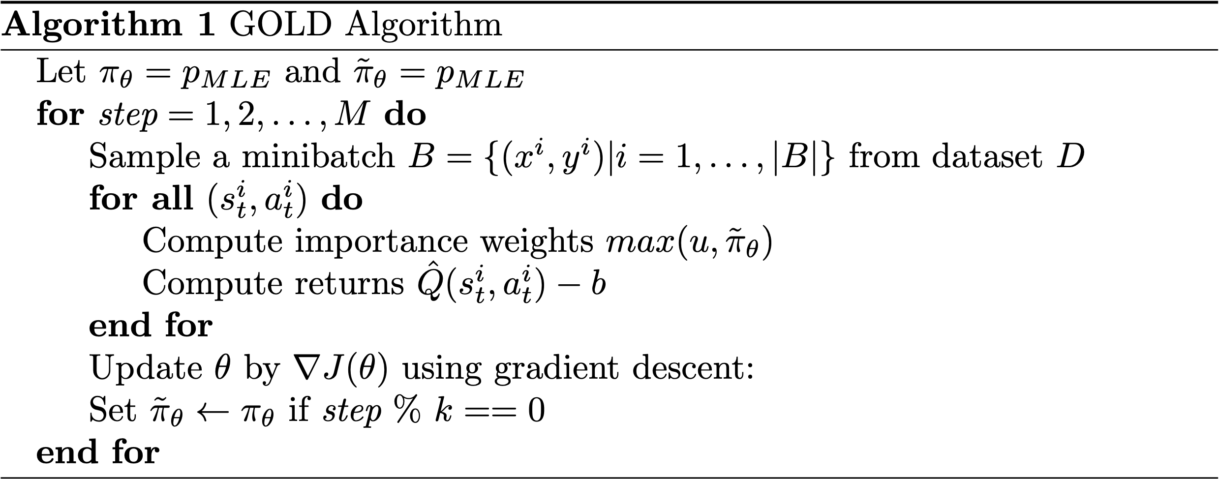
A few things to note in the above algorithm:

There are two policies. The first one is used for importance sampling and is denoted by $\pi_{b}$. The second one is the text generation policy that will be used for generating text during evaluation, denoted by $\pi_{\theta}$.
The minibatch $B$ is sampled from a dataset of demonstrations $D$. Each $(s_i^t, a_i^t)$ is constructed from a single demonstration $(x_i,y_i) \in D$ as follows: ($s_i^t = (y_{0:t-1}, x), a_i^t = y_t$). Thus, each demonstration will provide $T$ $(s_i^t, a_i^t)$ pairs.

How GOLD uses Importance Sampling

In offline RL, we are provided a set of demonstrations constructed from policy $\pi_{b}$, and we want to learn a policy $\pi_{\theta}$ given these demonstrations. One problem we have here is that the expected value of the return ${\hat Q}(s_t,a_t)$ is supposed to be computed using samples generated by $\pi_{\theta}$. However, we do not have these samples; rather, we have demonstrations generated by $\pi_{b}$. Thus, we utilize importance sampling to estimate the expectation of ${\hat Q}(s_t,a_t)$ under $\pi_{\theta}$ given samples from $\pi_{b}$.

The weight at index $t$ used by importance sampling is computed as:

\[\begin{align*} w_t = \prod_{t'=0}^{t}\frac{\pi_{\theta}(a_{t'}|s_{t'})}{\pi_{b}(a_{t'}|s_{t'})} \end{align*}\]

Intuitively, this captures the probability ratio between the learned policy and the behavioral policy for tokens $y_{0:t}$. However, there are two problems with this equation:

According to the paper, multiplying per-token importance weights for token indices $0$ to $t$ is sensitive to hyperparameters and takes longer to converge.
We do not know $b$, only the demonstrations constructed by it.

To address (1), we can estimate the weights using its per-token form: $w_t =\frac{\pi_{\theta}(a_{t}|s_{t})}{\pi_{b}(a_{t}|s_{t})}$. While this estimate is biased, it has been shown to reduce variance and works reasonably well if both $\pi_{b}$ and $\pi_{\theta}$ are close (Serban et al., 2017), (Levine et al., 2020). To address (2), we can estimate $\pi_{b}$, but the paper instead assumes a uniform distribution $\pi_{b}(\tau) \approx$ 1/N, making $\pi_{b}(a_{t}|s_{t})$ constant. This assumption implies that each demonstration in the dataset is equally likely, changing the importance weight to $w_t = \pi_{\theta}(a_{t}|s_{t})$. As we will see later in the post, GOLD performs well under the assumption that $\pi_{b}(\tau) \approx$ 1/N. However, it is uncertain what effect this assumption has on variance and bias in estimating the gradient. As such, one direction for future work would be to analyze this assumption. Interestingly, this assumption also has the knock-on effect of allowing the importance weights to represent the likelihood of the gold standard text under the model’s distribution. This then allows GOLD to use importance weighting as a way to guide the model to learn training samples with high likelihood under the model.

Reward Functions

The reward function $r_t = R(s_t, a_t)$ steers GOLD to find an optimal policy and thus has a large impact on the performance of a model trained by GOLD. Ideally, we want the reward function to represent the perceptual quality of text (how likely a human would have generated the text given a context) (Huszar, 2015), (Hashimoto et al., 2019), so that our learned policy generates text that a human would generate. To this end, three different reward functions are introduced which fall into two categories: sequence-level reward and token-level reward.

Sequence-level reward: This reward function only provides a reward if the entire demonstration constructed by the model is in the dataset (this does not make assumptions about the likelihood of the demonstrations in the dataset; all are equally likely):

\[R(s_t,a_t) := \begin{cases} 1 & \textit{if }(s_{0:T},a_{0:T}) \in D \wedge t == T \\ 0 & \textit{otherwise} \end{cases}\]

This function is sparse in that it will only be non-zero exactly $N$ times, where $N$ is the number of demonstrations in $D$. RL methods do not do well with sparse rewards as a reward of 0 does not provide any learning signal. Their experiments (summarized in MLE vs GOLD) even show that GOLD with this reward function (referred to as GOLD-$\delta$) performs worse than the reward functions that we describe next, which are less sparse.

Token-level reward: The previous reward function assumes all demonstrations in the dataset are equally likely. However, in text generation tasks, a context can have multiple correct outputs (e.g., if our context is a news article, there can be multiple, different correct summaries of it), each of which can be associated with a probability based on the tokens it contains. This implies then that a context’s reference (text that we want the model to generate) also has a probability associated with it.

To assign a probability to each of the references, we can use an approximation of text perceptual quality, specifically the MLE solution $p_{MLE}$. According to the paper, $p_{MLE}$ is a reasonable approximation to text perceptual quality when $p_{MLE}$ is restricted only to the demonstrations. Given this estimation, two reward functions are defined based on how they are applied to the value function ${\hat Q}(s_t,a_t)$:

${\hat Q}(s_t,a_t)$ is a product of probabilities: $R_p(s,a) := log~p_{MLE}(a|s)$ and ${\hat Q}(s_t,a_t) = \sum_{t’=t}^{T}\gamma^{t’-t} log~p_{MLE}(a_{t’}|s_{t’})$. A sequence will have high reward only if every token has a high likelihood under $p_{MLE}$. Thus, we can think of this as a “strict” reward in that there is no room for errors. GOLD with this reward function is referred to as GOLD-$p$ in the paper.
${\hat Q}(s_t,a_t)$ is a sum of probabilities: $R_s(s,a) := p_{MLE}(a|s)$ and ${\hat Q}(s_t,a_t) = \sum_{t’=t}^{T}\gamma^{t’-t} p_{MLE}(a_{t’}|s_{t’})$ A sequence can have high reward even if one of the tokens is not very likely under $p_{MLE}$ as the low-likelihood token will be marginalized out during summation. In contrast to (1), this reward is more lenient in that there is room for some errors. GOLD with this reward function is referred to as GOLD-$s$ in the paper.

Why GOLD does Offline RL vs Online RL

Online RL usually utilizes exploration methods to discover new courses of action in an environment. However, exploration can be detrimental for text generation as it may yield text that has zero reward (e.g., text that is syntactically incorrect). For example, if we have a news article that we want to summarize, exploration could yield summaries that are off-topic. Furthermore, the large action space in text generation makes exploration challenging as space of syntactically incorrect text is most likely larger than the space of syntactically correct text. Thus, we do not want any exploration, but we do want to keep as close as possible to the provided demonstrations.

Offline RL makes sense to use then as it focuses on learning a policy based only on demonstrations. Another advantage with offline RL is that the environment dynamics are known and deterministic in text generation (i.e., the transition from state $y_{0:t-1}$ to $y_{0:t}$ is done by appending $y_t$ to $y_{0:t-1}$). Thus, there is no need to interact with an environment to get the next state.

Training Objective

Recall that the training objective for policy gradient aims to find a policy that maximizes the expected cumulative reward:

\[J = max_{\pi_{\theta}}\mathbb{E}_{\tau \sim \pi_{\theta}} \Big[\sum_{t=0}^{T}\gamma^{t}r_t\Big]\]

Recall from Background that taking the gradient of this objective function yields the following (instead of $R(\tau)$, we have ${\hat Q}(s_t,a_t)$):

\[\nabla J(\theta)= \mathbb{E}_{\tau \sim \pi_{\theta}} \Big[\sum_{t=0}^{T} \nabla_{\theta}~log(\pi_{\theta}(a_t|s_t)){\hat Q}(s_t,a_t)\Big]\]

Adding the approximated importance sampling weight $\tilde{\pi}_{\theta}(s_t,a_t)$ yields the final gradient:

\[\nabla J(\theta)= \mathbb{E}_{\tau \sim \pi_{\theta}} \Big[\sum_{t=0}^{T} max(u, \tilde{\pi}_{\theta}(a_t|s_t))\nabla_{\theta}~log(\pi_{\theta}(a_t|s_t)){\hat Q}(s_t,a_t)\Big]\] \[\nabla J(\theta) \approx \sum_{i=0}^{|B|} \Big[\sum_{t=0}^{T} max(u, \tilde{\pi}_{\theta}(a^i_t|s^i_t))\nabla_{\theta}~log(\pi_{\theta}(a^i_t|s^i_t)){\hat Q}(s^i_t,a^i_t)\Big]\]

where the importance sampling weight is lower-bounded by $u$. One thing to note here is that the parameters for the policy used in importance sampling $\tilde{\pi}_{\theta}$ is kept frozen and thus is not updated by the gradient. This policy is, however, periodically updated to be the main policy $\pi_{\theta}$ in the GOLD algorithm. Another thing to note here is that ${\hat Q}$ and $\tilde{\pi}_{\theta}$ utilizes references from the demonstration dataset (i.e., $y_{0:t-1}$ from $s^i_t = (y_{0:t-1}, x)$ are references) while $\pi_{\theta}$ uses model-generated outputs (i.e., $y_{0:t-1}$ from $s^i_t=(y_{0:t-1}, x)$ are model-generated outputs).

MLE vs GOLD

GOLD was evaluated on four different language generation tasks: extractive summarization (simply called summarization in the original paper), extreme summarization, machine translation, and question generation. The below table provides a summary of the tasks used in the paper, and their corresponding datasets and metrics:

Task	Task Description	Dataset	Metric
Extractive Summarization (ESUM) (called CNN/DM in paper)	Generate a few sentence summary given a piece of text, where the sentences are extracted from the original text	CNN/DailyMail	ROUGE-1/2/L
Extreme Summarization (XSUM)	Generate a single sentence summary given a piece of text	BBC news	ROUGE-1/2/L
Machine Translation (MT)	Generate a translation of a given text in a particular language	IWSLT14 De-En	BLEU-4
Natural Question Generation (NQG)	Generate a question that can be answered by a short span of text found within a given passage	SQuAD QA	BLEU-4

We will mainly focus on the overall findings in this blog post. More specific experiment results can be found in the original paper.

MLE vs GOLD - Transformer and Non-Transformer Models

GOLD was first compared against MLE for two off-the-shelf non-Transformer models: NQG++ (Zhou et al., 2017) for NQG and Pointer Generator Network (PGN) (See et al., 2017) for extractive summarization (i.e., NQG++ and PGN were trained either with GOLD or MLE). Overall, their results indicated that NQG and PGN trained using GOLD will achieve better BLEU and ROGUE scores than MLE. One interesting thing to note here is that this improvement is at the cost of perplexity; for NQG, MLE had 29.25 compared to 158.45 for the GOLD-$s$ variant (lower perplexity is better). GOLD was then compared against two Transformer models: pretrained BART (Lewis et al., 2020) for NQG, and extractive and extreme summarization, and the original Transformer (Vaswani et al., 2017) for machine translation. Their results indicate that BART and the Transformer trained using GOLD will achieve better BLEU and ROGUE scores than MLE. Similar to the non-Transformer model, this performance gain is at the cost of perplexity.

MLE vs GOLD - Human Evaluation

In addition to the standard metrics in the literature, sentences generated by GOLD+BART were compared against MLE+BART from a human standpoint. The tasks used in these experiments were NQG, ESUM, and XSUM. Specifically, human evaluation was crowdsourced using Amazon Mechanical Turk, where 200 pairs of examples were created for each of the three tasks and each of the three tasks were done by 15 unique evaluators.

NQG Evaluation: Each evaluator was presented with a source paragraph, the questions generated by the MLE-trained model and GOLD-$s$-trained model, and the words in the paragraph that answered the generated questions. Each evaluator was then asked to determine which question was better, or if there was a tie.

ESUM/XSUM Evaluation: Each evaluator was presented with a reference summary of an article, and a summary generated by the MLE-trained model and GOLD-s-model. Each evaluator was then asked to determine which summary was closer in meaning to the reference summary.

Overall, their results indicate that the workers preferred the output generated via the GOLD-trained model compared to the MLE-trained model.

Addressing Exposure Bias + Train/Eval Mismatch

Recall the main goal of GOLD was to address two key problems with the MLE objective: training/evaluation metric mismatch and exposure bias. Let’s now go into how GOLD exactly addresses these.


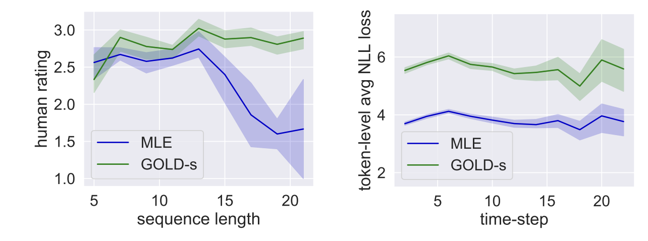
Exposure Bias Experiment from Paper (regions denote 95% confidence interval). Left: Text generation length vs. avg. human rating. Based on 736 samples from NQG task. Right: Time step vs. avg token-level negative log likelihood (NLL) of $t^{th}$ token given gold prefixes. Based on development dataset from NQG task. (Image source: (Pang and He, 2017, Page 7))

Exposure Bias: GOLD suffers less from exposure bias compared to MLE as it uses the history distribution induced by the model when training rather than the gold history. To test this hypothesis, an experiment is run on the NQG task, where text output quality between the two models as the output length increases is used as a proxy when measuring exposure bias. This output quality is computed by using the ratings of Amazon Mechanical Turk workers. The above figure (left) shows the results of this experiment. Their results indicate that the questions generated with GOLD do not suffer from quality degradation whereas MLE does. As model-generated data is used during inference, it is likely that the first few states would be quite similar to the gold history for models trained using MLE. However, as the model continues to generate output, the difference will accumulate and the model-generated distribution will deviate further and further away from the gold standard’s distribution. To verify that the performance drop is caused by exposure bias and not from other factors of long-sequence generation, the two models are also evaluated by being conditioned on gold histories during evaluation. This would zero out exposure bias, so both models should have similar performance across all time steps. The results for this experiment are also shown in the above figure (right). Their results indicate that the token-level negative log likelihood (NLL) losses remain stable across time steps for both MLE and GOLD, supporting the claim that exposure bias caused the performance degradation of MLE.


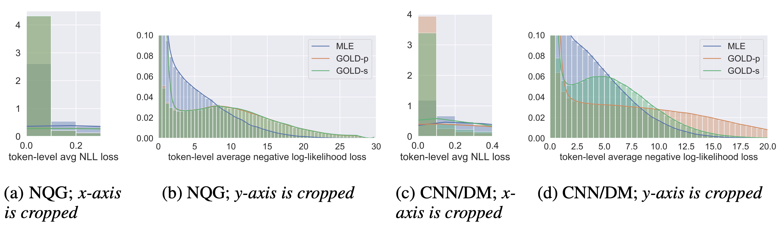Assessing Metric Mismatch Experiment from Paper. Left Two Figures: Histogram of token-level negative log likelihood (NLL) using standard models on development dataset from NQG task. Right Two Figures: Histogram of token-level NLL using standard models on development dataset from ESUM task (Image source: (Pang and He, 2017, Page 6))

Training/Evaluation Metric Mismatch: GOLD suffers less from training/evaluation mismatch compared to MLE. To test this hypothesis, an experiment is run on the NQG and ESUM tasks, where the distributions of token-level NLL loss is used to better understand the impact of this mismatch. Evaluation metrics encourage high precision (i.e., text generated from a model must be high quality); thus models that have high precision would be best matched with the evaluation metrics. The results for this experiment is shown in the above figure. Their results indicate that the NLL loss is spread out when training using MLE, which indicates that models trained using it try to generate all tokens in the vocabulary ((b) and (d) in the above figure). These results align with the idea that MLE encourages models with high recall, where the model is able generate more diverse text for a given context (i.e., it generates relevant text with irrelevant text for a given context). Their results also indicate that the NLL loss for models trained using GOLD are concentrated on near-zero losses ((a) and (c) in the above figure). These results actually align with the idea that GOLD encourages higher precision, where models trained using it generate a single text given a context (i.e., generates relevant text without irrelevant text for a given context). Thus, models trained using GOLD are better matched with evaluation metrics.

Concluding Remarks

This blog post provides a better understanding of the GOLD algorithm from the ICLR 2021 paper Text Generation by Learning from Demonstration, and an understanding of how RL is used in text generation. We hope this has been of help to researchers and practitioners in the field of RL and NLP.

We now look to provide some future research questions that we thought of during our survey of this work:

Can we steer GOLD to generate diverse text given a single context? - “Diverse” has several meanings. The paper goes into three different definitions, but we focus on one of them here: the ability to generate a variety of correct generations given one context. GOLD currently can produce high-quality text for a single context and different text given different contexts; however, it may not be able to provide high-quality diverse texts given a single context.
Can we apply contexts other than text to RL-based language generation models? - This paper focused mainly on textual context (e.g., source text for translation or articles for text summarization). However, there are definitely other non-textual contexts that can be used for text generation. Take for example an image which could be used for caption generation, or game states from computer games, which could be used to generate text for text-based game-playing or story generation.
Can we use GOLD to fine-tune NLG models to be more confident with unconfident tokens? - GOLD currently upweights confident tokens and downweights unconfident ones using importance weighting so a generation model can generate text with a bias towards confident tokens. This makes the model view the unconfident tokens as “noise,” when those tokens may just be uncommon tokens. For example, suppose we had tokens such as “wrote” and “authored.” If the model was more confident with “wrote” than “authored,” then the model would always generate “I wrote a blog post” rather than “I authored a blog post.”
Can we modify GOLD’s reward function to generate high-quality, socially-conscious text? - GOLD successfully used importance weighting and a reward function that approximated human perceptual quality of text as a guiding mechanism for generating high-quality text. This idea effectively shows that a reward function can be used to control what text is generated by a model, possibly allowing humans to guide generation models to construct high quality, socially acceptable text.

References

Iulian V Serban, Chinnadhurai Sankar, Mathieu Germain, Saizheng Zhang, Zhouhan Lin, Sandeep Subramanian, Taesup Kim, Michael Pieper, Sarath Chandar, Nan Rosemary Ke, Sai Rajeshwar, Alexandre de Brebisson, Jose M. R. Sotelo, Dendi Suhubdy, Vincent Michalski, Alexandre Nguyen, Joelle Pineau and Yoshua Bengio. A deep reinforcement learning chatbot. In Advances in Neural Information Processing Systems, pp. 1-9, 2017..