Discovering Non-Monotonic Autoregressive Ordering for Text Generation Models using Sinkhorn Distributions

25 Mar 2022 | autoregressive non-monotonic natural-language-generation sinkhorn-distributions Kumar, Ashutosh

Natural-Language-Generation (NLG) is a process for producing a sequence of natural language tokens. While the input to the NLG pipeline includes, but is not limited to, audio, video, image, structured documents, and natural language itself, the output is restricted to human readable texts.

Neural NLG models typically comprise a neural network, called an encoder, for converting inputs to points in vector spaces and a decoder (Decoding Strategies), that uses the encoded representations, for producing tokens (which can be words, characters or subwords). These tokens, after post-processing, are combined to form a human-readable natural language text.

While the primary target audience for this blog are researchers in NLG, anyone with an interest in knowing about or exploring a new research topic in NLG should find this insightful.

Since the main focus of this blog is on decoding strategies and a very specific problem in the same domain, we start with an overview of the standard practices in decoding.

Decoding Strategies

Autoregressive Generation: The most conventional approach for obtaining outputs from a decoder is through something called Autoregressive Generation. In this, the decoder utilizes information obtained from the encoder as well as the previous sequentially generated tokens, to produce a new token. Early papers [Uria 2016, Germain 2015, Vinyals 2015] showed that the order in which the tokens are generated is critical for determining the best autoregressive sequence. However, owing to the simplicity and intuitiveness of using the standard left-to-right order, they became ubiquituous. The paper (as well as this blog) is an attempt to restore the interest in analysing different ordering schemes for autoregressive token generation. The two main ordering schemes under autoregressive decoding are:

Monotonic Ordering: A pre-determined order of sequence generation, be it left-to-right or right-to-left, is referred to as monotonic ordering. Mathematically, the modeling objective is: $$ p(\mathbf{y} \vert \mathbf{x}) = p(y_1 \vert \mathbf{x}) \prod_{i=2}^n p(y_i \vert y_{<i}, \mathbf{x}) $$ Note that the ordering information is implicit in this formulation. It is assumed that the best ordering of sequence to be generated is known.
Adaptive Non-Monotonic Ordering : In the most general cases, determining the order of prediction of generated tokens is helpful for obtaining an optimal final sequence $\mathbf{y}$. More formally, the modeling objective for such an approach is: $$ p(\mathbf{y}, \mathbf{z} \vert \mathbf{x}) = p(y_{z_1} \vert \mathbf{x})p(z_1 \vert y_{z_1}, \mathbf{x})\prod_{i=2}^n p(y_{z_i} \vert z_{<i}, y_{z_{<i}}\mathbf{x})p(z_i \vert z_{<i}, y_{z_{\leq i}}\mathbf{x}) $$ where $\mathbf{z} = (z_1, \ldots, z_n) \in S$ is a one-dimensional representation of permutation. Although mathematically sound, determining the best order using previous known approaches is empirically challenging, especially in situations where the domain of the data is not provided. The model needs to infer that *adaptively* from the data.

Decoding

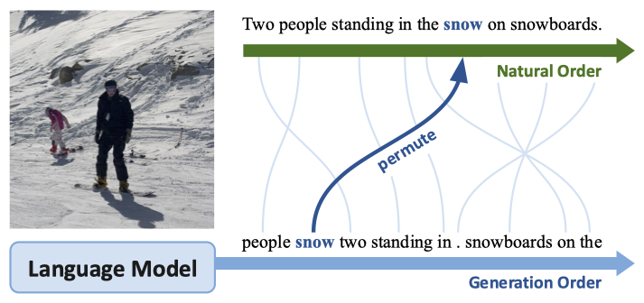
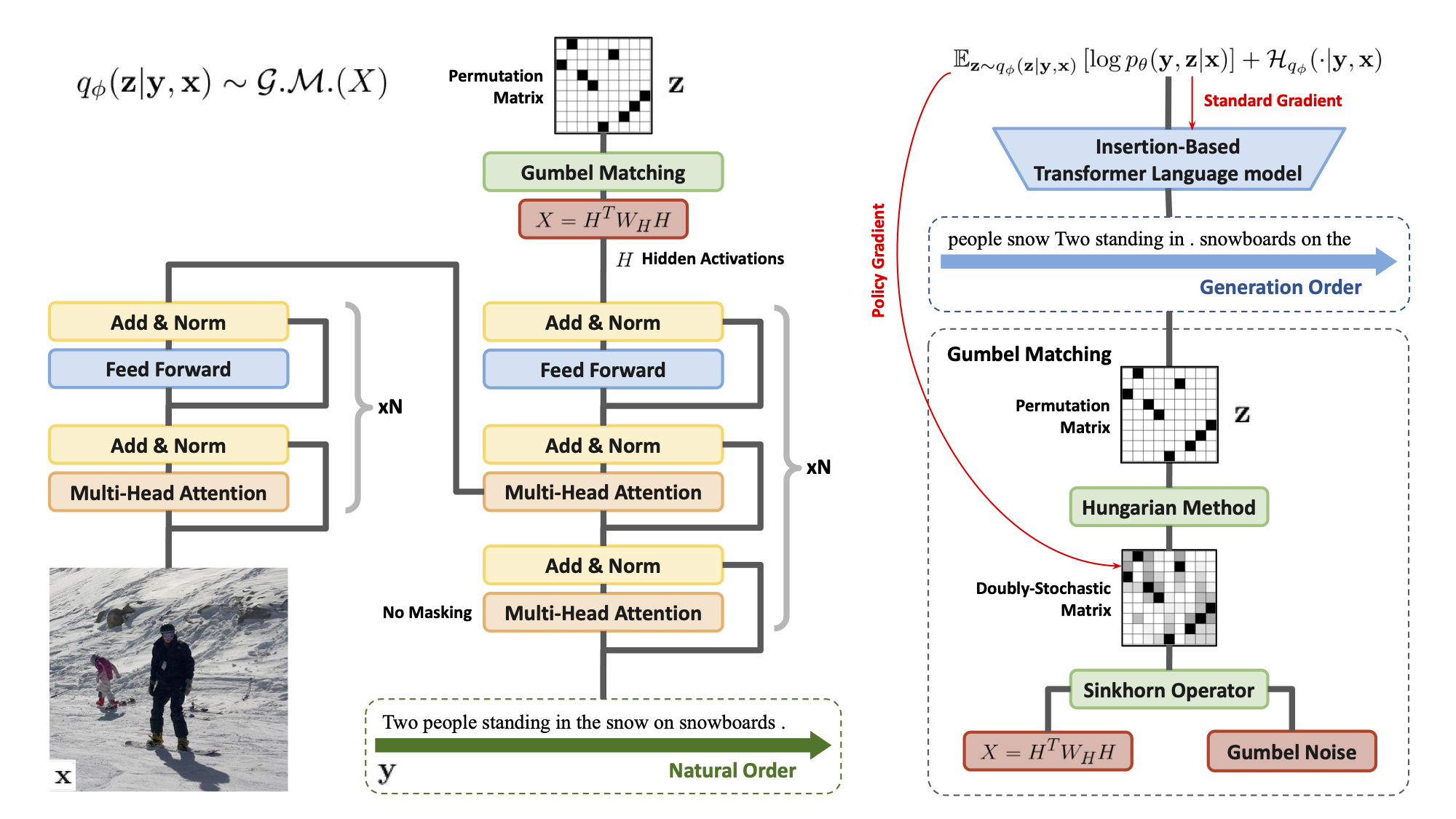
In the above figure the top autoregressive strategy (natural order) is that of monotonic left-to-right ordering, while the lower one (generation order) is that of adaptive non-monotonic ordering. It can be seen that in the adaptive non-monotonic strategy the more descriptive tokens or content words like people, now are produced before fillers and determiners like on, the. Note that the generated tokens are permuted (automatically based on the ordering $\mathbf{z}$) to form the natural order in case of non-monotonic ordering strategy, for grammaticality (Image Source: Li 2021).

While being empirically superior in terms of quality, auto-regressive generations are time-inefficient. Each token is predicted sequentially and in the case of Non-Monotonic and adaptive ordering the number of time-steps doubles with every new output token since the location is also being predicted apart from the actual token of generation itself. To address this issue of time-inefficiency, another set of techniques were developed under the umbrella term non-autoregressive generation.

Non-Autoregressive Generation: These approaches decode multiple tokens in parallel but under certain conditional-independent constraints. While being time-efficient, the quality of generations of these sequences is lower as compared to auto-regressive approaches. Most of the work focusing on Non-Autoregressive approaches, typically tries to alleviate the inaccuracies introduced due to the conditional-independence between tokens constraint. This blog discusses the paper [Li 2021] that utilizes one such method to obtain a good set of non-monotonic, adaptive orderings to guide the final autoregressive token generation model.

In this post, we will be focusing on one of the lesser explored area - Non-Monotonic Autoregressive Order (NMAO) in Decoding. In particular, we will be discussing the ICLR 2021 paper “Discovering Non-monotonic Autoregressive Orderings with Variational Inference” [Li 2021], the background needed for understanding the work as well as the way-forward.

Table of Content

What is the main focus of this paper?
Background
What are Sinkhorn Networks ?
How are Non-Monotonic Autoregressive Orderings (NMAO) discovered using Sinkhorn Networks ?
Show Me Some Experiments and Results
- Quantitative Results
- Qualitative Results
What Next ?
Conclusion and TL;DR

What is the main focus of this paper?

The primary aim of this work is to produce high-quality token sequences. An intermediate important step in this is to generate an optimal ordering for guiding autoregressive token generation models. To generate optimal ordering, the paper proposes a domain-independent unsupervised non-autoregressive learner based on Sinkhorn Networks. The key contributions of this paper are:

Propose an encoder architecture that conditions on training examples to output autoregressive orders using techniques in combinatorial optimization.
Propose Variational Order Inference (VOI) that learns an approximate posterior over autoregressive orders.
Develop a practical algorithm for solving the resulting non-differentiable Evidence Lower Bound Objective (ELBO) end-to-end with policy gradients.

In this blog, we will break down each of the contributions and also discuss the results as well as future research directions. Being a technically dense paper, it is imperative to develop a certain level of mathematical maturity. To that end, we provide the necessary mathematical background in the next section.

2. Background

In this section, we develop the mathematical background necessary for understanding and appreciating the technical contributions of this work. If you are familiar with it kindly [Click here to go to section 4]

We start with some special matrices and operations.

(A) Special Matrices, and Operations

Permutation Sequences and Permutation Matrix

A Permutation sequence is arrangement of elements of a set into any sequence. Mathematically, it is a function $\sigma: S \to S$, where S is any set, such that every element occurs exactly once as an image value. One such example is $\sigma_i({1,3,5,2,4}) = (3,2,1,5,4)$. A set of all such permutations on [$1, \ldots, n$] is denoted as $\mathcal{S}_n$.

Permutation Matrices ($P$) are square binary matrices having exactly one entry as 1 in each row and each column and 0 elsewhere. A set of all such permutation matrices is denoted as $\mathcal{P}_{n \times n}$.

It can easily be seen that there exists a natural bijection between $\mathcal{S}_n$ and $\mathcal{P}_{n \times n}$. The equivalence between Permutation matrices and sequences can best be understood through an example. Let us consider an $n$-dimensional vector (or sequence) $\mathbf{a} = (a_1, a_2, a_3, a_4)$, and we apply a permutation $\sigma$ to get $(a_2, a_1, a_4, a_3)$ i.e., $\sigma(a_1, a_2, a_3, a_4)=(a_2, a_1, a_4, a_3)$. The corresponding permutation matrix $P \in \mathcal{P}_{n \times n}$ for this is $\begin{bmatrix} 0 & 1 & 0 & 0 \\ 1 & 0 & 0 & 0 \\ 0 & 0 & 0 & 1 \\ 0 & 0 & 1 & 0 \end{bmatrix}$

This is because:

\[\begin{bmatrix} 0 & 1 & 0 & 0 \\ 1 & 0 & 0 & 0 \\ 0 & 0 & 0 & 1 \\ 0 & 0 & 1 & 0 \end{bmatrix} \begin{bmatrix} a_1\\ a_2\\ a_3\\ a_4 \end{bmatrix} = \begin{bmatrix} a_2\\ a_1\\ a_4\\ a_3 \end{bmatrix} = \sigma(a_1, a_2, a_3, a_4)\]

Matrix permanents $\text{perm}(X)$ and Bethe permanents $\text{perm}_B(X)$

Let us recall first the definition of a determinant of a matrix before moving to matrix permanents.

Consider a matrix: $X \in \mathbb{R}_{n \times n}$. The matrix determinant of $X$ is defined as:

\[\texttt{det}(X) = \sum_{\sigma \in S_n} \left( \texttt{sgn}(\sigma)\prod^{n}_{i=1}X_{i, \sigma_i}\right)\]

where $\texttt{sgn}(\sigma)$ equals $+1$ if $\sigma$ is an even permutation and equals $−1$ if $\sigma$ is an odd permutation.

The matrix permanent is similar in formulation, but without the $\texttt{sgn}$ operator. Formally,

\[\texttt{perm}(X) = \sum_{\sigma \in S_n} \prod^{n}_{i=1}X_{i, \sigma_i}\]

While determinants find applications in combinatorics as well as have geometric interpretations (volume of an $n$-dimensional parallelepiped), a matrix permanent is mainly used as a combinatorial object and has no such geometric interpretations.

For a special case of non-negative entries i.e., $X \in \mathbb{R}^+_{n \times n}$ (this will be useful for us later in VOI), the permanent can be approximated by solving a certain Bethe free energy optimization problem [Yedidia 2001]. The Bethe permanent is an approximation for a matrix $X \in \mathbb{R}^+_{n \times n}$ and is defined as:

\[\texttt{perm}_B(A) = \texttt{exp}\left(\max_{\gamma \in \mathcal{B}_{n \times n}} \sum_{i, j}\left(\gamma_{i,j}\log X_{i,j} - \gamma_{i,j}\log \gamma_{i,j} + (1-\gamma_{i,j})\log (1-\gamma_{i,j})\right)\right)\]

where $\mathcal{B}_{n \times n}$ is a doubly-stochastic matrix i.e., a matrix whose each entry is a non-negative real number and each row and each column sums to 1. For e.g., $\begin{bmatrix} \frac{7}{12} & 0 & \frac{5}{12} \\ \frac{2}{12} & \frac{6}{12} & \frac{4}{12} \\ \frac{3}{12} & \frac{6}{12} & \frac{3}{12} \end{bmatrix}$

Since bethe permanent is an approximation, we should be aware of its upper and lower bounds w.r.t. the matrix permanent [Votobel 2010]. Note that the following inequality holds:

\[\sqrt{2}^{-n} \texttt{perm}(A) \leq \texttt{perm}_B(A) \leq \texttt{perm}(A)\]

Now that we have defined all these special types of matrices, it is a good time to talk about Birkhoff Polytopes which is useful for understanding Sinkhorn Networks, and the rest of the blog.

Birkhoff Polytopes:

The Birkhoff polytope $\mathcal{B}_n$ is the convex polytope in $R^{n \times n}$ whose points are the doubly stochastic matrices. This polytope has $n!$ vertices and by the Birkhoff–von Neumann theorem it follows that each vertex is a permutation matrices. Further more, any doubly-stochastic matrix can be represented as a convex combination of permutation matrices.

By definitions of permutation matrices, and doubly-stochastic matrices it should be evident that $\mathcal{P}_{n \times n} \subset \mathcal{B}_{n \times n} \subset \mathbb{R}^+_{n \times n}$

(B) Prelude to Gumbel-Sinkhorn

Definition: Frobenius Norm

Given two matrices $A$ and $B$, the Frobenius norm: $\langle A,B \rangle_F = Tr(A^\top B) = \sum_{ij}\overline{A_{ij}}B_{ij}$

Discrete Approximations for Vectors

We build upon the Sinkhorn operators through an analogy of softmax for permutations.

1. Normalization - Softmax Operator: One way to approximate discrete classes from continuous values is using a temperature-dependent softmax function, defined component-wise as: $\texttt{softmax}_\tau(x)_i = \frac{\texttt{exp}(x_i/\tau)}{\sum_j\texttt{exp}(x_j/\tau)}$. For $\tau > 0$, $\texttt{softmax}_\tau(x)$ is a point in the probability simplex i.e., a set of vector points such that the co-ordinate wise sum of each of those vectors is 1. It is also known that as $\tau \to 0$, $\texttt{softmax}_\tau(x) \to \texttt{one-hot}(x)_i$, i.e., a binary vector containing only one $1$ entry at the argmax of $\texttt{softmax}_\tau(x)$ and $0$, elsewhere.

2. Maximization Problem: Finding $\texttt{one-hot}(x)_i$ can be cast as a maximization problem i.e., $\text{argmax }{x_i}=\text{argmax}_{s\in\mathcal{S}_n}\langle x,s\rangle$, where $\mathcal{S}_n$ is a set of all $n$-dimensional permutations, defined earlier. In essence, we start with a normalization of a vector ($\texttt{softmax}$ operation), then cast the $\texttt{one-hot}$ permutation vector finding as a linear-maximization problem.

Sinkhorn Operations: Discrete Approximations for Matrices

Moving to two-dimensions i.e., vectors to matrices, we do a similar thing. We first define a normalization operator (called Sinkhorn Operator), and then formulate the problem of finding a permutation matrix as a linear-maximization problem. An equivalent temperature dependent Sinkhorn operator helps in a discrete approximation of continuous values in a Birkhoff polytope.

1. Normalization - Sinkhorn Operator: Let $X \in \mathbb{R}_{n \times n}$ and $A \in \mathbb{R}^+_{n \times n}$. A Sinkhorn operator is an iterative construct defined as follows:

\[S^0(X) = \exp(X) \\ S^l(X) = \mathcal{T}_c(\mathcal{T}_r(S^{l-1}(X))) \\ S(X) = \lim_{l \to \infty}S^l(X),\]

where $\mathcal{T}_c = A \oslash (A\mathbf{1}_N\mathbf{1}_N^\top)$ and $\mathcal{T}_r = A \oslash (\mathbf{1}_N\mathbf{1}_N^\top A)$. Here $\oslash$ represents element-wise division, and $\mathbf{1}_N$ is the vector of all $1$s. Informally, iterative application of $\mathcal{T}$ results in normalizing a non-negative matrix along columns and rows.

Important: It is interesting to note that $S(X)$ belongs to the Birkhoff polytope i.e., it is necessarily a doubly-stochastic matrix. [Sinkhorn 1964]

2. Maximization Problem: Finding a $\texttt{one-hot}$ vector in two-dimensions is equivalent to finding a permutation matrix. This too can be cast as a maximization problem involving matrix $X$ as follows:

\[M(X) = \text{argmax}_{P \in \mathcal{P}_N} \langle P, X\rangle_F\]

here $M(\cdot)$ is called the matching operator.

Like softmax, a temperature-dependent Sinkhorn operator also has some similar interesting properties when $\tau \to 0$. But first we need to understand that the temperature-dependent Sinkhorn operator $S(X/\tau)$ solves a certain entropy-regularized problem in the Birkhoff polytope $\mathcal{B}_n$.

Theorem 1

For a doubly-stochastic matrix $P$, having entropy as: $h(P) = - \sum_{i, j}P_{ij}\log P_{ij}$,

\[S(X/\tau) = \text{argmax}_{P \in \mathcal{B}_N} \langle P, X\rangle _F + \tau h(P)\]

and under certain assumptions regarding the entries of $X$ (see Mena 2018) , the following convergence holds:

\[M(X) = \lim_{\tau \to 0^+} S(X/\tau)\]

where M(X) is a permutation matrix from the Birkhoff Polytope.

In practice, since taking limits for the Sinkhorn operator on $l$ is infeasible, a truncated version of the Sinkhorn operator is considered ($l \to L$ where $L \in \mathbb{N}$).

(C) Jensens’ Inequality

For a convex function $f$ the following inequality (Jensens’ Inequality) holds:

\[f(\mathbb{E}(X)) \leq \mathbb{E}(f(x)),\]

where $\mathbb{E}(X)$ is the Expectation over the random variable $X$. It can be intuitively understood through the following diagram. Here $f$ is a univariate function over $X$. Functional value of the Expectation (black line) is less than the Expectation value of the function (magenta/pink line)

(Image Source: Convex Functions)

(D) Log Trick

In policy gradient algorithms, we are required to compute gradients of the Expected Value of Logs. A clever replacement trick helps in deriving the gradient, easily. The following is for the discrete random variable, however a similar results holds true for continuous random variables.

Let $\mathbb{E}_{q_\phi}[\log(p_\theta) - b]$ be the expected value of $\log(p_\theta) - b$ under the distribution $q_\phi$. Here $b$ (will be useful and referred to as baseline formulation in Optimization Procedure) is a constant. Then the derivative of it w.r.t. $\phi$ is,

\[\begin{split} \nabla_\phi \mathbb{E}_{q_\phi}[\log(p_\theta) - b] &= \nabla_\phi \sum(\log(p_\theta) - b).q_\phi\\ &= \sum(\log(p_\theta)-b).\nabla_\phi q_\phi \end{split}\]

We know that the following holds

\[\begin{split} &\nabla_\phi \log(q_\phi) &= \frac{1}{q_\phi}. \nabla_\phi q_\phi \\ \implies &\nabla_\phi q_\phi &= q_\phi(\nabla_\phi \log(q_\phi)) \end{split}\]

Replacing the value of $\nabla_\phi q_\phi$ in the previous equation, we get

\[\begin{split} \nabla_\phi \mathbb{E}_{q_\phi}[\log(p_\theta) - b] &= \sum(\log(p_\theta) - b).q_\phi \nabla_\phi \log(q_\phi)\\ &= \mathbb{E}_{q_\phi}[(\log(p_\theta) - b).\nabla_\phi \log(q_\phi)] & \\ \text{We know that } \nabla_\phi \mathbb{E}_{q_\phi}[\log(p_\theta) - b] &= \nabla_\phi \mathbb{E}_{q_\phi}[\log(p_\theta)] & (\because b \text{ is a constant}) \\ \implies \nabla_\phi \mathbb{E}_{q_\phi}[\log(p_\theta)] &= \mathbb{E}_{q_\phi}[(\log(p_\theta) - b).\nabla_\phi \log(q_\phi)] & \\ \end{split}\]

Now that we have developed a certain understanding of the mathematical background, let’s discuss Sinkhorn Networks. These networks form one of the main components for finding good non-monotonic autoregressive orderings.

3. What are Sinkhorn Networks ? [Optional Reading]

This section is optional and the reader may jump to the Gumbel-Sinkhorn Summary Table directly, if they wish to. We put it here for completeness, since it forms the encoder network in the VOI model [Click here to go to section 4]

Sinkhorn Networks (Mena 2016) are supervised models for learning to reconstruct scrambled objects or permutations $\tilde{X}$ given a set of training examples ($X_i, \tilde{X_i}$).

Sinkhorn Networks

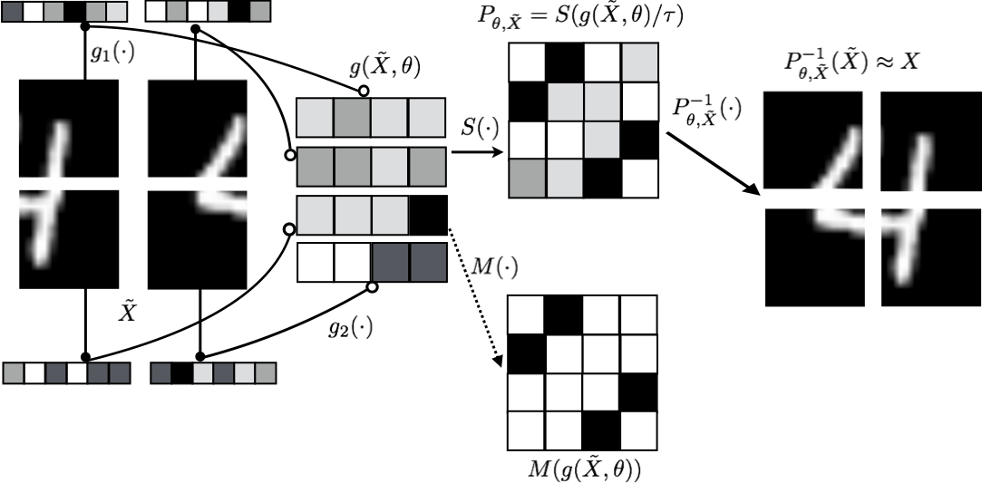
From the above figure (Image Source: Mena 2018) it can be seen that the original distorted input $\tilde{X}$ goes through transformations $g, g_1, g_2$. The its output is then passed through the temperature-dependent Sinkhorn operator $S(\cdot)$ during training, and the matching operator $M(\cdot)$ during inference. $S(\cdot)$ can be thought of as a soft-permutation. Here, $P_{\theta, \tilde{X}}$ (in the ideal case) is a permutation matrix mapping $X \to \tilde{X}$. Unlike traditional neural networks where output changes with any change in the input, Sinkhorn networks are only dependent on the content of the input and not the order in which they are presented to the network.

This entails that we should only consider those networks that satisfy the following property of permutation equivariance i.e., $P_{\theta, P'\tilde{X}}(P'\tilde{X}) = P'(P_{\theta, \tilde{X}}\tilde{X})$, where $P'$ is any arbitrary permutation matrix.

The main goal of a sinkhorn network is to solve permutation problems like the jigsaw puzzle given in the diagram above or sorting a set of $N$ numbers. Therefore, it naturally fits into the paradigm of finding good orderings for autoregressive generations and will be leveraged by VOI (Variational Order Inference). VOI will not have access to the ground truth $X$ for learning good networks although it will have access to gradients based on the final objective of the model, which is to generate high-quality sequences.

While being technically sound, there is another aspect which needs to be understood before moving to the main model - Gumbel-Sinkhorn and Gumbel-Matching distributions.

The best way to go about it is through an analogy with the ubiquituous Gumbel-Softmax. In computational graphs containing stochastic nodes i.e., latent probabistic representations, Kingma and Welling (2014) proposed the reparameterization trick viz the gumbel trick. Since reparameterisation is not directly differentiable, sampling under a softmax approximation is considered [Jang 2017]. A similar construction is done for Sinkhorn networks where we would want to sample from the Gumbel-Matching Distribution (gumbel-dependent distribution for the matching operator). The Gumbel-softmax is replaced with the Gumbel-Sinkhorn distribution and sampling is done through it (we will see this in the algorithm for VOI). Without going into complete mathematical details about each step, we state the following useful theorem and the associated table for easy reference.

Theorem 2

Let $X \in \mathbb{R}_{n \times n}, \tau > 0$. The $\textbf{Gumbel-Sinkhorn distribution } \mathcal{G.S.}(X,\tau)$ is defined as follows:

\[\mathcal{G.S.}(X,\tau) = S \left(\frac{X+ \epsilon}{\tau}\right)\]

where $\epsilon$ is a matrix of i.i.d standard Gumbel noise. Then $\mathcal{G.S.}(X,\tau) \overset{\text{a.s}}{\to} \mathcal{G.M.}(X)$ as $\tau \to 0^+$. $\mathcal{G.M.}(X)$ is the Gumbel-Matching distribution.

Since we would want to ideally sample from $\mathcal{G.M.}(X)$, which makes the backpropagation through the network infeasible directly, a good strategy would be to first sample from $\mathcal{G.S.}(X,\tau)$ and approximate sample from $\mathcal{G.M.}(X)$ by taking $\tau \to 0^+$. For more information on a.s or almost sure convergence, please refer [3].

The following table is helpful in understanding the analogy between Gumbel-softmax and Gumbel Sinkhorn Distribution

	Classes/Categories	Permutations
Polytope	Probability Simplex $\mathcal{S}$	Birkhoff polytope $\mathcal{B_N}$
Linear program Approximation	$\text{argmax }{x_i}=\text{argmax}_{s\in\mathcal{S}}\langle x,s\rangle$ $\text{argmax}_i x_i = \lim_{\tau\rightarrow 0^+} \text{softmax}(x/\tau)$	$M(X)=\text{argmax}_{P\in\mathcal{B}}\left< P,X\right>_F$ $M(X) = \lim_{\tau\rightarrow 0^+} S(X/\tau)$
Entropy Entropy regularized linear program	$h(s)=\sum_i -s_i \log s_i $ $ \text{softmax}(x/\tau)=\text{argmax}_{s\in\mathcal{S}}\langle x,s\rangle +\tau h(s)$	$h(P)=\sum_{i,j}-P_{i,j}\log\left(P_{i,j}\right)$ $S(X/\tau)=\text{argmax}_{P\in\mathcal{B}}\left< P,X\right>_F +\tau h(P)$
Reparameterization Continuous approximation	$\textbf{Gumbel-max trick}$ $\text{argmax}_i (x_i+\epsilon_i)$ $\textbf{Concrete}$ $\text{softmax}((x+\epsilon)/\tau)$	$\textbf{Gumbel-Matching }\mathcal{G}{M}(X)$ $M(X+\epsilon)$ $\textbf{Gumbel-Sinkhorn }\mathcal{G}{S}(X,\tau)$ $S((X+\epsilon)/\tau)$

4. How are NMAO discovered?

The key highlight of the paper is to use variational inference combined with partial Sinkhorn networks for discovering non-monotonic ordering of sequences which in turn is used for generating high-quality autoregressive tokens.

We first formulate the problem, and then discuss the proposed model with an inference framework called Variational Order Inference(VOI). In VOI, we will find out that the Sinkhorn distributions play an important role in sampling good orderings $\mathbf{z}$ (defined in formulation).

Formulation

Consider a sequence of source tokens (or source representations in case of non-text input domains) $\mathbf{x} = (x_1, \ldots, x_m)$. The goal of an NLG model is to model a sequence of target tokens $\mathbf{y} = (y_1, \ldots, y_n)$, conditioned on $\mathbf{x}$.

In the standard autoregressive modeling with fixed orderings (monotonic auto-regressive), the model is formulated as follows:

\[p(\mathbf{y} \vert \mathbf{x}) = p(y_1 \vert \mathbf{x}) \prod_{i=2}^n p(y_i|y_{<i}, \mathbf{x})\]

In this work, however, the focus is on modeling non-monotonic autoregressive NLG frameworks, where the position or ordering of the sequence token is not fixed. Let the latent variable to model these orderings be denoted as $\mathbf{z} = (z_1, \ldots, z_n)$. Each $z_i$ denotes the position at which $y_{z_i}$ should be inserted into the sequence $\mathbf{y}$. Thus instead of modeling $p(\mathbf{y} \vert \mathbf{x})$ directly, we are interested in modeling $p(\mathbf{y}, \mathbf{z}\vert\mathbf{x})$ first and marginalizing it over $\mathbf{z}$ to obtain $p(\mathbf{y} \vert \mathbf{x})$. In order to model this autoregressively, $p(\mathbf{y}, \mathbf{z}\vert\mathbf{x})$ is factorized as follows:

\[p(\mathbf{y}, \mathbf{z} \vert \mathbf{x}) = p(y_{z_1}\vert\mathbf{x})p(z_1 \vert y_{z_1}, \mathbf{x})\prod_{i=2}^n p(y_{z_i} \vert z_{<i}, y_{z_{<i}}\mathbf{x})p(z_i \vert z_{<i}, y_{z_{\leq i}}\mathbf{x}),\]

Note that $y_{z_i}$ denotes that the $i^{th}$ generated token needs to be put in position $z_i$ of the output sequence, and $\mathbf{z} \in \mathcal{S}_n$, where $\mathcal{S}_n$ is a set of permutations of {1, $\ldots$, n}. In practice, the approach does not first create a fixed-length sequence of blanks and then replace the blanks with actual values. Instead, it adopts an insertion-based approach, and dynamically inserts a new value at a position relative to the previous values (using similar approaches as Pointer Networks). We use position $\mathbf{r}$ relative to the previous generated values instead of $\mathbf{z}$. Since there is a bijection between $\mathbf{r}$ and $\mathbf{z}$ , for simplicity, we still use throughout the blogpost / paper.

Variational Order Inference

The ultimate goal of any NLG model is to obtain high-quality generations conditioned on the original source values. Mathematically, one would like to maximize the likelihood of obtaining output sequence $\mathbf{y}$ i.e., maximize $\mathbb{E}_{(x,y)\sim\mathcal{D}}[\log p_\theta(\mathbf{y}\vert\mathbf{x})]$. Simplifying it further in terms of latent variable orders $\mathbf{z}$ and variational inference, we get the following:

\[\mathbb{E}_{(x,y) \sim \mathcal{D}}[\log p_\theta(\mathbf{y} \vert \mathbf{x})] = \mathbb{E}_{(x,y) \sim \mathcal{D}} \log \left[ \mathbb{E}_{z \sim q_\phi (\mathbf{z} \vert \mathbf{y}, \mathbf{x})} \left[ \frac{p_\theta(\mathbf{y}, \mathbf{z} \vert \mathbf{x})}{q_\phi(\mathbf{z} \vert \mathbf{x}, \mathbf{y})} \right] \right]\]

We know that “$\log$” is a concave function. Therefore “$-\log$” is a convex function. Now applying the Jensen’s inequality on inner $\log$ and $\mathbb{E}$ in the RHS, we get

\[\mathbb{E}_{(x,y) \sim \mathcal{D}} \log \left[ \mathbb{E}_{z \sim q_\phi (\mathbf{z}|\mathbf{y}, \mathbf{x})} \left[ \frac{p_\theta(\mathbf{y}, \mathbf{z} \vert \mathbf{x})}{q_\phi(\mathbf{z} \vert \mathbf{x}, \mathbf{y})} \right] \right] \geq \mathbb{E}_{(x,y) \sim \mathcal{D}} \left[ \mathbb{E}_{z \sim q_\phi (\mathbf{z}\vert\mathbf{y}, \mathbf{x})} \left[ \log p_\theta(\mathbf{y}, \mathbf{z} \vert \mathbf{x}) \right] + \mathcal{H}_{q_\phi}( \cdot \vert \mathbf{y}, \mathbf{x}) \right] \\ \mathbb{E}_{(x,y) \sim \mathcal{D}}[\log p_\theta(\mathbf{y}\vert\mathbf{x})] \geq \mathbb{E}_{(x,y) \sim \mathcal{D}} \left[ \mathbb{E}_{z \sim q_\phi (\mathbf{z} \vert \mathbf{y}, \mathbf{x})} \left[ \log p_\theta(\mathbf{y}, \mathbf{z} \vert \mathbf{x}) \right] + \mathcal{H}_{q_\phi}( \cdot \vert \mathbf{y}, \mathbf{x}) \right]\]

We call the right hand side the main objective or $\texttt{ELBO}$. This is the Evidence Lower Bound that needs to be maximized. In other words, we will be using gradient ascent i.e., $\theta = \theta + \alpha_\theta g_\theta$ and $\phi = \phi + \alpha_\phi g_\phi$, where $\alpha$ are the learning rates, $\phi, \theta$ are network parameters and $g$ are the corresponding gradients of $\texttt{ELBO}$ w.r.t the network parameters.

Let us understand this diagrammatically via computational graphs to develop better intuitions. Consider the following figure.

VOI

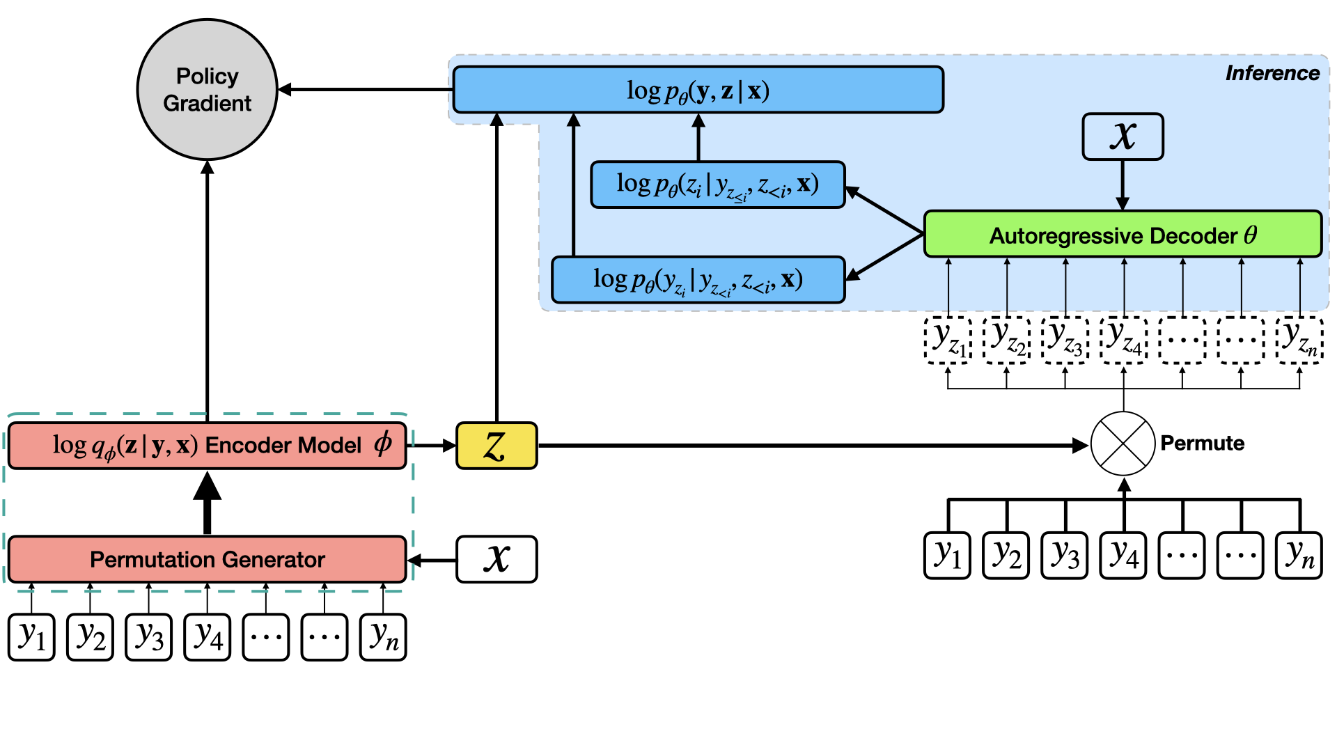
$\mathbf{y}$ is taken in its natural order and passed through a non-autoregressive network ($\phi$ and the permutation generator (pink)) along with the source value $\mathbf{x}$ and outputs the latent order $\mathbf{z}$ (yellow) in the forward pass. $\theta$ (green) takes in the source value $\mathbf{x}$ and predicts both $\mathbf{y}$ as well as the ordering sequence in which the tokens of $\mathbf{y}$ need to appear (in blue).

[IMPORTANT] Caveat: The encoder $\phi$ is in part a Sinkhorn network (albeit without the ground truth order sequence - this is learned from the main objective of the model $p(\mathbf{y}, \mathbf{z} \vert \mathbf{x})$ through policy gradients), while the decoder $\theta$ is a fully-differentiable sequence-to-sequence network (in this paper, the transformer network [Vaswani 2017, Gu 2019] - which itself has an encoder and a decoder).

The main objective is jointly optimized for $\theta$ and $\phi$. It should be noted that only the decoder $\theta$ is useful during inference/testing (See the blue highlighted portion in the main figure). $\phi$ is therefore an assistive network for obtaining high-quality orderings to correctly guide the decoder $\theta$ towards finally producing high-quality generations.

Optimization Procedure

As discussed before, we will be using gradient ascent i.e., $\theta = \theta + \alpha_\theta g_\theta$ and $\phi = \phi + \alpha_\phi g_\phi$, where $\alpha$ are the learning rates, $\phi, \theta$ are network parameters and $g$ are the corresponding gradients of $\texttt{ELBO}$ w.r.t the network parameters. Let’s find out the gradients w.r.t each network parameter.

Gradients for the Decoder Network ($\theta$):

Gradient update for $\theta$ is done using the Monte Carlo gradient estimate. First sample $K$ latent ordering $\mathbf{z}_1, \ldots, \mathbf{z}_K$ from $\phi$ (pink in the diagram). Notice in the main objective that $\theta$ appears only in the first term on the RHS. And then the update happens on $\theta$ using the following gradient estimate:

\[g_\theta = \mathbb{E}_{y \sim \mathcal{D}} \left[ \frac{1}{K} \sum_{i=1}^K \nabla_\theta \log p_\theta (\mathbf{y}, \mathbf{z}_i \vert \mathbf{x}) \right]\]

Note that $\mathbf{z}_i$ is an entire permutation sequence, and not the $i^{th}$ co-ordinate of a permutation sequence.

Gradients for the Encoder Network ($\phi$) and finding optimal ordering:

Although this network would play no role in the final inference model, it does provide the most useful information based on which the decoder $\theta$ learns to generate high-quality sequences. The discrete nature of $\mathbf{z}$ makes it impossible for gradients to flow from the blue network ($\log p_\theta(\mathbf{y}, \mathbf{z} \vert \mathbf{x})$) to the yellow one ($\phi$).

Owing to the complexity of this step, we break it down into 2 Stages:

Stage 1 : The MDP Formulation

In order to make gradient (backpropagation) flow tractable, the main objective is formulated as a one-step Markov decision process having the following constituent parameters (State space: $\mathcal{S}$, Action space: $\mathcal{A}$, Reward function: $\mathcal{R}$):

State Space: $\mathcal{S} = (\mathbf{x}, \mathbf{y}) \in \mathcal{D}$
Action Space: $\mathcal{A} = S_{\text{length}(\mathbf{y})} \text{ with entropy }\mathcal{H}_{q_\phi}( \cdot \vert \mathbf{y}, \mathbf{x})$
Reward function: $\mathcal{R} = \log p_\theta(\mathbf{y}, \mathbf{z} \vert \mathbf{x})$

Let’s consider the main objective again. It is found that adding an coefficient to the entropy term with annealing, speeds up the convergence of the decoder network. We now derive the gradient of the main objective w.r.t. the encoder network parameters $\phi$. Because of an MDP formulation, described above, this gradient will be useful as a policy gradient step. Notice that the method involves baseline formulation ($b(\mathbf{y}, \mathbf{x})$), which is independent of $z$, and the log trick

\[\begin{split} g_\phi &= \mathbb{E}_{(\mathbf{x},\mathbf{y}) \sim \mathcal{D}} \left[ \mathbb{E}_{\mathbf{z} \sim q_\phi (\mathbf{z} \vert \mathbf{y}, \mathbf{x})} \left[ \nabla_\phi \log q_\phi(\mathbf{z} \vert \mathbf{y}, \mathbf{x}) (\log p_\theta(\mathbf{y}, \mathbf{z} \vert \mathbf{x}) - b(\mathbf{y}, \mathbf{x})) \right] + \beta.\nabla_\phi\mathcal{H}_{q_\phi}( \cdot \vert \mathbf{y}, \mathbf{x}) \right] \end{split}\]

However, it is to be noted that $b$ is not taken with respect to the whole dataset and is state space ($\mathbf{x}, \mathbf{y}$) dependent. This is done to normalize the reward scale difference across state space, reducing gradient variance and stabilizing the training. Empirically [Li 2021]. find that this significantly stabilizes training. In particular,

\[b(\mathbf{y}, \mathbf{x}) = \mathbb{E}_{z \sim q_\phi}[\log p_\theta(\mathbf{y}, \mathbf{z}_i \vert \mathbf{x})]\]

This, can again be estimated using the Monte-Carlo estimates

\[b(\mathbf{y}, \mathbf{x}) \approx \frac{1}{K}\sum_{i=1}^K\log p_\theta(\mathbf{y}, \mathbf{z}_i \vert \mathbf{x})\]

Stage 2: Closed form of $q_\phi(\mathbf{z} \vert \mathbf{y}, \mathbf{x})$

Stage 2.a: Closed form of $q_\phi(\mathbf{z} \vert \mathbf{y}, \mathbf{x})$ - The Numerator

Having developed an intuition about the gradient RL formulation, we now proceed to discuss one of the critical components of the gradient update - Obtaining a closed form for the distribution $q_\phi(\mathbf{z} \vert \mathbf{y}, \mathbf{x})$. In order to understand this, let us recall our preliminaries on Permutation-Matrices, Birkhoff-Polytopes, and Gumbel-Sinkhorn. We know that $\mathcal{P}_{n \times n} \subset \mathcal{B}_{n \times n} \subset \mathbb{R}^+_{n \times n}$ and a natural bijection occurs between the the set of permutation matrices $\mathcal{P}_{n \times n}$ and the set of permutation vectors $\mathcal{S}_n$.

Let us consider a function $f_n : \mathcal{S}_n \to \mathcal{P}_{n \times n}$ where $f_n(\mathbf{z})_i = \texttt{one-hot}(z_i)$. Now since $z \in \mathcal{S}_n$, $q_\phi(\mathbf{z} \vert \mathbf{y}, \mathbf{x}) = q_\phi(f_n(\mathbf{z}) \vert \mathbf{y}, \mathbf{x})$. We now proceed with modeling the distribution $q_\phi( \cdot \vert \mathbf{y}, \mathbf{x})$. This is exactly the Gumbel-Matching distribution $\mathcal{G}.\mathcal{M}.(X)$ over $\mathcal{P}_{n \times n}$ we defined earlier, where $X = \phi(\mathbf{y}, \mathbf{x}) \in \mathbb{R}^{n \times n}$. Now for $P \in \mathcal{P}_{n \times n}$,

\[q_\phi(\mathbf{z} \vert \mathbf{y}, \mathbf{x}) = q_\phi(f_n^{-1}(P) \vert \mathbf{y}, \mathbf{x}) = q_\phi(P \vert \mathbf{y}, \mathbf{x}) \propto \texttt{exp} \langle X, P \rangle_F\]

Note that $\texttt{exp} \langle X, P \rangle_F$ is only the numerator for the closed of $q_\phi(\mathbf{z} \vert \mathbf{y}, \mathbf{x})$. We will discuss about the denominator and final update in Stage 2.b

To obtain samples in $\mathcal{P}_{n \times n}$ from the Gumbel-Matching distribution, relax $\mathcal{P}_{n \times n}$ to $\mathcal{B}_{n \times n}$ by defining the Gumbel-Sinkhorn distribution $\mathcal{G}.\mathcal{S}.(X, \tau)$. Based on Theorem 1, we know that as $\tau \to 0^+$, $\mathcal{G}.\mathcal{S}.(X, \tau) \overset{\text{a.s}}{\to} \mathcal{G}.\mathcal{M}.(X)$. For more information on a.s or almost sure convergence, please refer 3]. After relaxation, to approximately sample from $\mathcal{G}.\mathcal{M}.(X)$, first sample from $\mathcal{G}.\mathcal{S}.(X, \tau)$ and then apply the Hungarian Algorithm

Stage 2.b: Closed form of $q_\phi(\mathbf{z} \vert \mathbf{y}, \mathbf{x})$ - The Denominator

We have already seen that the numerator of $q_\phi(\mathbf{z} \vert \mathbf{y}, \mathbf{x}) = \texttt{exp} \langle X, P \rangle_F$, which is tractable. However, the denominator is $\sum_{P \in \mathcal{P}_{n \times n}}\texttt{exp} \langle X, P \rangle_F$ i.e., a summation over all permutation matrices which is intractable since there are $n!$ permutation matrices in $\mathcal{P}_{n \times n}$. Let us first see what it looks like:

\[\begin{split} q_\phi(\cdot \vert \mathbf{y}, \mathbf{x}) &= \sum_{P \in \mathcal{P}_{n \times n}}\texttt{exp} \langle X, P \rangle_F \\ &= \sum_{\sigma \in S_n} \texttt{exp}\left(\sum_{i=1}^n X_{i, \sigma(i)}\right)\\ &= \sum_{\sigma \in S_n} \prod_{i=1}^n \left(\texttt{exp}(X)\right)_{i, \sigma(i)}\\ &= \texttt{perm}\left(\texttt{exp}(X)\right) \end{split}\]

We take the help of Bethe permanents defined earlier, and approximate $\sum_{P \in \mathcal{P}_{n \times n}}\texttt{exp} \langle X, P \rangle_F$ as Bethe permanents.

Having finally obtained the closed form solution of $q_\phi(\mathbf{z} \vert \mathbf{y}, \mathbf{x})$, we can optimize $\phi$ using gradient ascent (since we want to maximize $\texttt{ELBO}$) by applying $g_\phi$.

Taking care of the large permutation space

We have seen that $q_\phi(\mathbf{z} \vert \mathbf{y}, \mathbf{x})$ is tremendously complex and requires a lot of computations. A natural question here is: Why go through all this, if the ultimate goal is to just get better final sequences? $p_\theta(\mathbf{y}, \mathbf{z} \vert \mathbf{x})$. Infact, we won’t even be using the $\phi$ model during inference. While the approximation using Bethe permutation makes $q_\phi(\mathbf{z} \vert \mathbf{y}, \mathbf{x})$ tractable, it needs to be established whether the overall quality of generations would actually become better. We describe that in a few lines here.

In practice, if $p_\theta(\mathbf{y}, \mathbf{z}^* \vert \mathbf{x}) \geq p_\theta(\mathbf{y}, \mathbf{z} \vert \mathbf{x}) \forall z \in S_n$ then $p_\theta(\mathbf{y}, \mathbf{z} \vert \mathbf{x})$ increases as the edit distance between $\mathbf{z}$ and $\mathbf{z}^*$ decreases, where $\mathbf{z}^*$ is the optimal ordering of the sequence.

This is what the final update procedure looks like

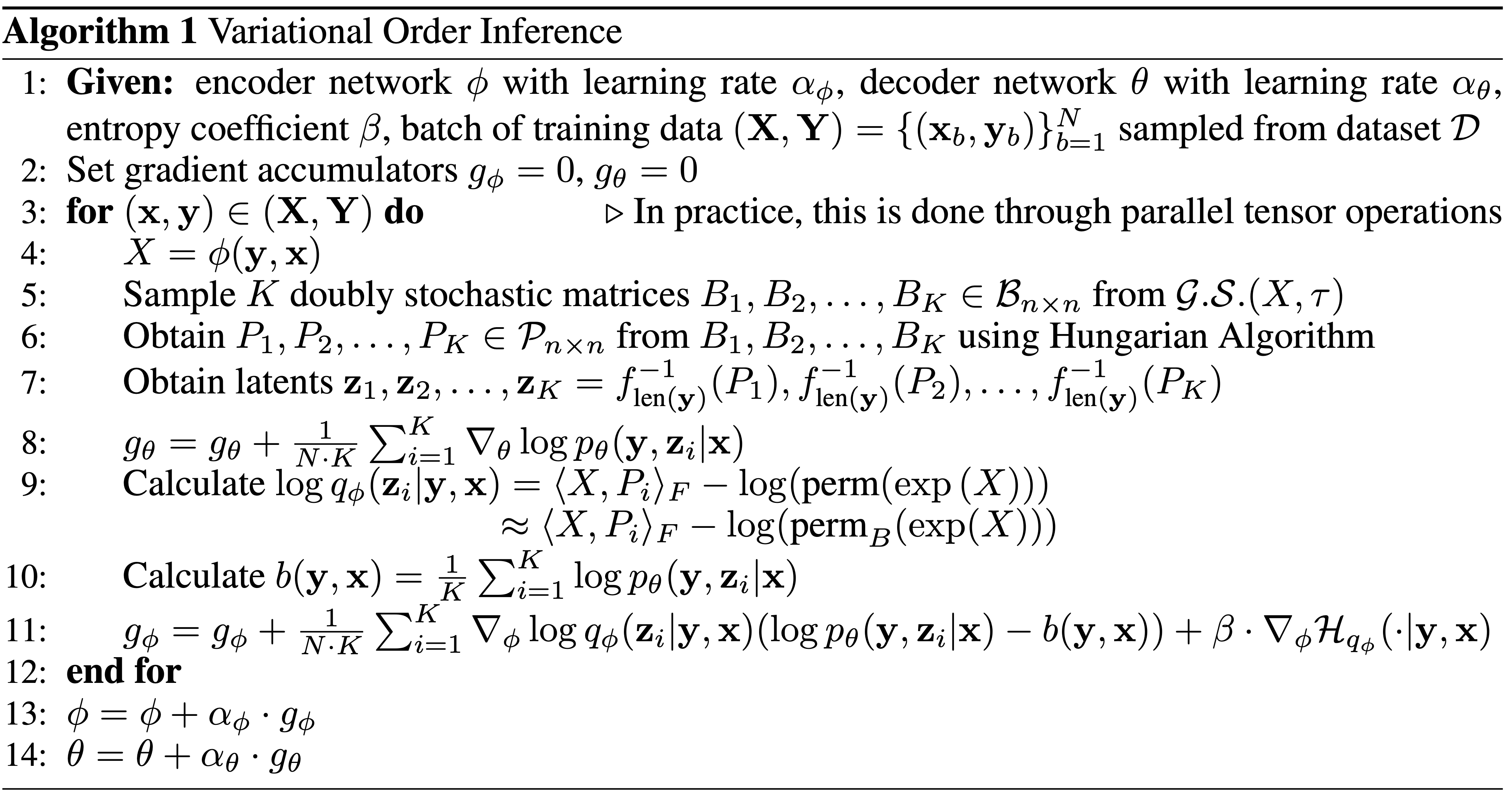VOI Algorithm (Image Source: Li 2021)

Once the model has been trained, we need to generate autoregressive sequences. This is descibed in the following sub-section.

Inference

As had been previously discussed, $\phi$ is just an assistive network and will be discarded during inference. The main goal of $\phi$ is to find a latent order which maximized the probability of $p_\theta(\mathbf{y}, \mathbf{z} \vert \mathbf{x})$. The decoder model (which is in fact a full sequence-to-sequence transformer network) takes an input source value (image, text, etc) and outputs the corresponding text auto-regressively, predicting the sequence tokens as well as the orderings. As alluded to earlier, the source value is $\mathbf{x}$, the output from the autoregressive decoder is $\mathbf{y}$ through ordering $\mathbf{z}$. In practice, $\mathbf{y}$ is generated through insertion, and the insertion order is parameterized by $\mathbf{z}$ (by first converting $\mathbf{z}$ to $\mathbf{r}$).

In the next section, we discuss the experiments conducted in the paper and the results obtained.

5. VOI in practice

VOI_practice (Image Source: Li 2021)

In this section, we discuss the findings of running VOI on different NLG tasks. Without going into the exact experimental details regarding each, we discuss only the key findings of the work. We categorize them into the following headings.

A. Quantitative Results

Baselines

Before moving to the quantitative results, we give a brief overview of the baselines that the model is compared with. In this section Ours refers to the model (mainly the decoder $\theta$) proposed in the original paper [Li 2021].

InDIGO - SAO[Gu 2019]: Previous state-of-the-art baseline in adaptive ordering strategy.
Ours - Random: Random ordering + Decoder
Ours - L2R [Wu 2018]: Left-to-right Ordering (standard ordering) + Decoder
Ours - Common [Ford 2018]: Common-First order is defined as generating words with ordering determined by their relative frequency from high to low + Decoder
Ours - Rare [Ford 2018]: Reverse of Common-First ordering + Decoder
Ours - VOI [Li 2021]: This work with non-autoregressive ordering prediction using Sinkhorn Networks + Decoder

Order	Image Captioning				Code Generation		Text Summarization			Machine Translation
	MS-COCO				Django		Gigaword			WMT16 Ro-En
	BLEU	METEOR	R-L	CIDEr	BLEU	Accuracy	R-1	R-2	R-L	BLEU	METEOR	TER
InDIGO - SAO	29.3	24.9	54.5	92.9	42.6	32.9	--	--	--	32.5	53.0	49.0
Ours - Random	28.9	24.2	55.2	92.8	21.6	26.9	30.1	11.6	27.6	--	--	--
Ours - L2R	30.5	25.3	54.5	95.6	40.5	33.7	35.6	17.2	33.2	32.7	54.4	50.2
Ours - Common	28.0	24.8	55.5	90.3	37.1	29.8	33.9	15.0	31.1	27.4	50.1	53.9
Ours - Rare	28.1	24.5	52.9	91.4	31.1	27.9	34.1	15.2	31.3	26.0	48.5	55.1
Ours - VOI	31.0	25.7	56.0	100.6	44.6	34.3	36.6	17.6	34.0	32.9	54.6	49.3

The above table presents the quantitative results for 4 different tasks (each with an associated dataset). The metrics being used are task-specific. It can be seen that VOI seems to be performing better than the baselines in all the tasks, thereby establishing itself as an effective model.

In addition to this, the paper also reports faster training run-times compared to its baseline InDIGO [Gu 2019]. This is expected because VOI outputs latent orderings non-autoregressively in a single forward pass while InDIGO searches for the orderings sequentially. Also, the search time increases with the length of the final sequence for InDIGO while it remains constant for VOI.

B. Qualitative Results

In this section we try to answer three interesting questions:

Question 1. Does the generation order of tokens convey anything about the sentence and the VOI model?

Generation Order (Image Source: Li 2021)

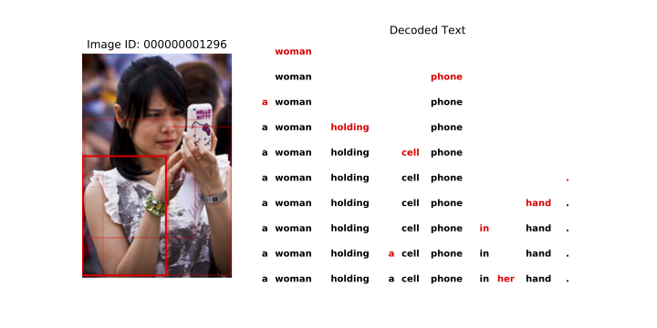
The key insight here is that the model generates the sentence in the following order: What to write about $\to$ How to write it

In the above figure, the tokens are generated in a top-down fashion. It can be seen that the inference model generates descriptive tokens like nouns, numerals, adverbs, verbs, adjectives e.g., “woman, phone”, first, while the uninformative text fillers like “in, a, her” are generated at the end. It is similar in some ways to how humans think about sentences, where what to write about precedes how to write it.

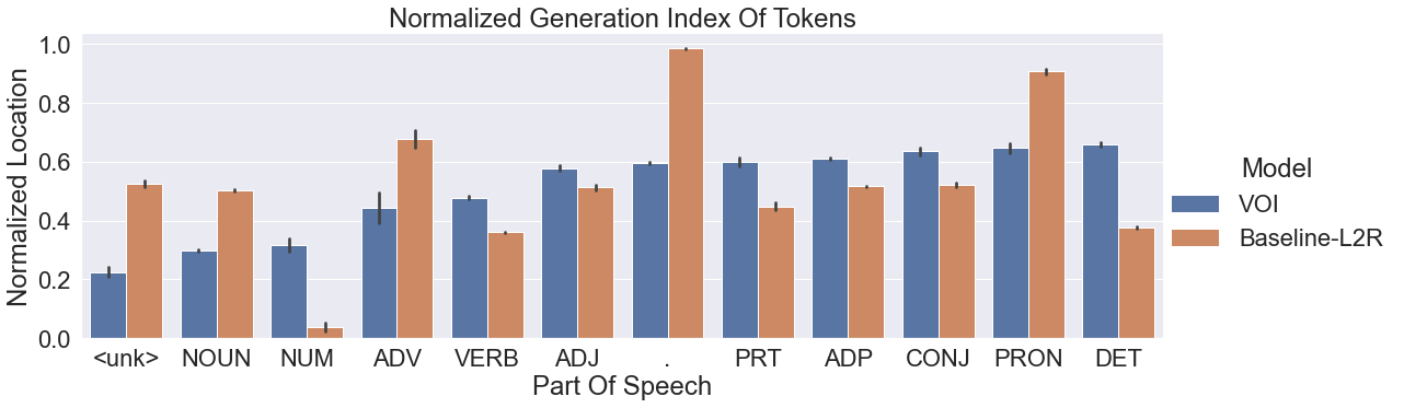
This behaviour can also be seen in the following diagram based on the overall dataset statistics.

Local Analysis (Image Source: Li 2021)

Here it can be seen that the VOI model favours nouns, numerics, adverbs much before pronouns and determiners, as we had seen already. This is in contrast to baseline-L2R ordering where determiners and conjunctions statistically appear much before descriptive tokens like nouns.

Question 2. Does the model generate orderings other than the standard left-to-right order? If not, it might be computationally wasteful to use this scheme.

While the local analysis showed that descriptive words are favoured, this does not fully merit a full understanding of the order strategy that was learned. In general, we want to see if a fixed ordering strategy is favoured over an adaptive strategy.

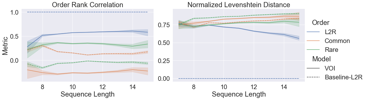
To address this, the author compare the orderings $\mathbf{w}, \mathbf{z}$ for the same output sequence $\mathbf{y}$. The two metrics used for this analysis are Normalized Levenshtein Distance $\mathcal{D}_{\text{NLD}} = \frac{\text{lev}(\mathbf{w}, \mathbf{z})}{n}$, where $n$ is the length of $\mathbf{y}$, and the correlation between the two orderings $\mathcal{D}_{\text{ORC}}(\mathbf{w},\mathbf{z})$.

Global Analysis (Image Source: Li 2021)

In the above figure, we see the comparison between VOI learned (adaptive) orders and a set of predefined orders (solid lines). The reference is an L2R fixed ordering model with the same set of predefined orders (dashed lines).

The figure leads to two observations:

It can be seen that although the VOI model favours left-to-right orderings, $\mathcal{D}_{\text{ORC}}(\mathbf{w},\mathbf{z}) = 0.6$ shows that left-to-right ordering might not be the perfect strategy. A non-zero value for rare-orderings also indicates that sometimes a more complex ordering strategy might be followed to obtain the high-quality generations $\mathbf{y}$.
Interestingly, as the generated sequences increase in length, $\mathcal{D}_{\text{NLD}}$ keeps on decreasing till the final value of 0.57. This shows that approximately half of the tokens (but not all) are already arranged according to a left-to-right generation order. The authors hypothesize that certain phrases might be getting generated from left-to-right, but their arrangement follows a best-first strategy. In other words, the model prefers generation of key semantic phrases, with the correct order of tokens in them, over filler/non-descriptive phrases.

Question 3. To what extent is the generation order learned by Variational Order Inference dependent on the contents of the conditioning variable $\mathbf{x}$? In other words is it adaptive?

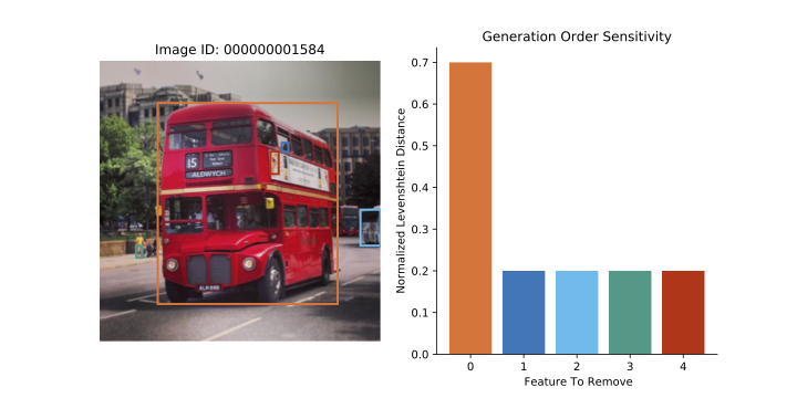Effect of Perturbation (Image Source: Li 2021)

With reference to the above figure, VOI first obtains generations $\mathbf{y}$, and its generation order $\mathbf{z}$ based on the original source image $\mathbf{x}$. In the next stage, keeping the generation $\mathbf{y}$ fixed, features are selectively removed from the image $\mathbf{x}$ (colored bounding boxes) and consequently a new generation-order $\mathbf{w}$ is inferred for each new image $\mathbf{x}'$. It is observed that through this operation, the original generation-order $\mathbf{z}$ and the new generation-order $\mathbf{w}$ differ from each other which results in non-zero edit distance when measured in terms of Normalized Levenshtein Distance ($\mathcal{D}_{\text{NLD}}$) between $\mathbf{z}$ and $\mathbf{w}$. In the above figure, when the Bus is removed from the image the corresponding change in $\mathcal{D}_{\text{NLD}}$ is as much as $0.7$. This shows that the model learns an adaptive strategy to produce generation-orders.

6. What Next?

The first thing would be to get hands on experience with the official code available at https://github.com/xuanlinli17/autoregressive_inference. Handling of the entropy function $\mathcal{H}_{q_\phi}( \cdot \vert \mathbf{y}, \mathbf{x})$ is an interesting aspect within the code which hasn’t been discussed here. Interested readers are also advised to go through Appendix B.3 in [Mena 2018] to know how the value of entropy is approximated. Dabbling with the code-base would give an opportunity to not only assess the strengths of the model, but also its limitations.

It was interesting to see that the proposed model worked really well in terms of computational speed as well as generation quality. This work paves way to a lot of follow up work. Some good research question worth looking at are:

In this paper, token sequence $\mathbf{y}$ is generated before ordering sequence $\mathbf{z}$. What would happen if $\mathbf{z}$ is generated before the $\mathbf{y}$?
Can such an approach be useful for other domains like image generation ?
Is it possible to develop a non-autoregressive decoder model for generating $\mathbf{y}$ ? Although non-autoregressive models are typically non-monotonic, it might be interesting to see if there is a substantial speed up in terms of inference times.
While being useful for conditional text generation, can such an approach help or be inducted into open-text-generation problems (Language Modeling with a twist)?
Are there any other such combinatorial optimization models (like Sinkhorn Networks), that might help in producing optimal orders?
From a theoretical and an analytical perspective, it might be interesting to see if there exists a unique optimal ordering or is there a set of plausible orderings - all leading to the same high-quality final output.

7. Conclusion

In the blog post we did the following:

Discussed various decoding strategies - monotonic autoregressive, non-monotonic autoregressive ordering and briefly shed light on non-autoregressive ordering [Go to Top]
Developed a comprehensive mathematical background especially the Sinkhorn Operator which is a Matrix equivalent of softmax operator which works on vectors. [Go to Background]
Gave a brief introduction to Sinkhorn Networks and noted that they are useful for jigsaw puzzle problems. [Go to Sinkhorn Networks]
Sinkhorn Networks were used for predicted non-monotonic autoregressive ordering, which ultimately helped in predicting orderings akin to how humans would think about a sentence. [Go to NMAO discovery]
Deep dive into Variational Order inference and the Optimization procedure. We connected all the necessary background, and Sinkhorn networks to finally get a model that is able to generate high-quality texts. [Go to VOI], [Go to Optimization Procedure]
Discussed the performance of VOI model, and saw that they are faster as compared to other non-monotonic autoregressive models, as well as more intuitive and high performing. [Go to Results]
Dabbled with some future research directions in this domain. [Go to What Next?]

TL;DR

We discussed an important but less researched topic - Discovering non-monotonic orderings for guiding models to obtain high-quality texts. We specifically discussed the model proposed in the ICLR 2021 paper by Li 2021. This model uses Gumbel-Sinkhorn distributions to assist a decoder model by providing good-quality generation orders during training. The trained models helped in generating high-quality outputs for four important NLG tasks: (a) Image Captioning (b) Code Generation (c) Text Summarization and (d) Machine Translation. Interestingly, the model behaviour replicated human behaviour in some sense - Considering what to write about, before figuring out how to write about it.

Errata/Incomplete formulation in the main paper:

Normalized Levenshein Distance - Equation (6): For two generation orders $\mathbf{w}, \mathbf{z} \in S_n$: $$ \begin{split} \text{lev}(\mathbf{w}, \mathbf{z}) &= \begin{cases} \color{red}{|\mathbf{w}|} & \color{red}{\text{if } |\mathbf{z}| = 0}\\ \color{red}{|\mathbf{z}|} & \color{red}{\text{if } |\mathbf{w}| = 0}\\ \color{red}{\text{lev}(\text{tail}(\mathbf{w}), \text{tail}(\mathbf{z}))} & \color{red}{\text{if } \mathbf{w}[0] = \mathbf{z}[0]}\\ 1 + \text{min}\begin{cases} \text{lev}(\text{tail}(\mathbf{w}), \mathbf{z}) \\ \text{lev}(\mathbf{w}, \text{tail}(\mathbf{z})) \\ \text{lev}(\text{tail}(\mathbf{w}), \mathbf{z}) \end{cases} & \text{otherwise} \end{cases} \\ \mathcal{D}_{\text{NLD}} (\mathbf{w}, \mathbf{z}) &= \frac{\text{lev}(\mathbf{w}, \mathbf{z})}{n} \end{split} $$
Equation (7): $$\mathcal{D}_{\text{ORC}}(\mathbf{w},\mathbf{z}) = 1 - 6. \sum_{i=0}^n \frac{(\mathbf{w}_i-\mathbf{z}_i)\color{red}{^2}}{(n^3-n)}$$

References

[15] Diederik P Kingma, Max Welling. Auto-Encoding Variational Bayes. ICLR, 2014