Euclidean geometry meets graph, a geometric deep learning perspective

25 Mar 2022 | graphs geometric-deep-learning Wang, Zichen, Amazon Web Services; Shi, Yunzhi, Amazon Web Services; Chen, Xin, Amazon Web Services

Graph neural networks (GNN) have been an active area of machine learning research to tackle various problems in graph data. A graph is a powerful way of representing relationships among entities as nodes connected by edges. Sometimes nodes and edges can have spatial features, such as 3D coordinates of nodes and directions along edges. How do we reason over the topology of graphs while considering those geometric features? In this post, we discuss Learning from Protein Structure with Geometric Vector Perceptrons (Jing et al. 2021), published in ICLR 2021.

Graphs and geometric graph

A graph is a common data structure using nodes connected by edges to represent complex relationships among entities. Nodes and edges usually have features on them for GNNs to learn from. Sometimes nodes and edges can have some spatial features, such as 3D coordinates of nodes and directions along edges, adding a layer of geometric relationships (including distance, direction, angle, etc.) among the entities. In this post, we term this type of graph with geometric feature vectors on nodes and/or edges as geometric graph.

Small molecules, macro-molecules, and geospatial data are all examples where one can construct geometric graphs: small molecules can be represented by a graph of atoms connected by chemical bonds, where atoms can be described by their coordinates in the 3D Euclidean space and chemical bonds can be described by vectors along their directions. The angles between adjacent chemical bonds are known to be indicative of the chemical properties of the molecule such as stability. Similarly, macro-molecules such as proteins can be represented by graphs of amino acid residues connected based on their spatial proximity. Each amino acid residue contains $k$ key atoms, allowing the node’s vector feature to be $\mathbf{V}_n \in \mathbb{R}^{k \times 3}$. Spatial networks and transportation networks can be constructed by treating intersections as nodes and roads as edges from urban geospatial data. Furthermore, the geographic coordinates of the intersections and the directions of the roads can be encoded as vector features on nodes and edges, respectively.

A Geometric Deep Learning perspective

The term “geometry” in a narrow sense is equivalent to the classic Euclidean geometry. However, other schools of geometries exist, such as Riemannian geometry. To unify the divergent schools of geometries, the Klein’s Erlangen Program views geometry as a study of invariance with respect to various transformations.

In the broader sense of geometry, a graph is also an important geometric object because its nodes are invariant to permutations: the ordering of its nodes does not change the property of the entire graph. At a local level, the ordering of direct neighbors does not affect a node’s attributes such as degree and centrality. With this perspective, when we impose Euclidean geometric features onto a graph to form a geometric graph, it is further invariant to Euclidean group transformations, $E(n)$, including rotations, translations and reflections.

Geometric Deep Learning (Bronstein et al. 2021) unifies many deep learning methods such as convolutional neural networks and GNNs by applying the principles in Erlangen geometry including symmetry and invariance. The Geometric Deep Learning blueprint provides three key building blocks for designing neural networks for new geometric objects: (i) a local equivariant map, (ii) a global invariant map, and (iii) a coarsening operator. In a typical GNN context, these building blocks correspond to layers that compute node-wise features, local pooling layers, and the final readout layer as a global pooling. This blueprint has the right level of generality to be used across a wide range of geometric domains depending on their symmetry groups, while providing a rich function approximation space with prescribed invariance and stability properties. In order to develop an effective geometric deep learning algorithm on geometric graphs, one needs to invent equivariant and invariant layers with respect to permutation and $E(n)$ symmetry groups. This can be achieved by extending the GNN to operate in $E(3)$ symmetries (assuming we are dealing with 3D Euclidean space).

Introducing the geometric vector perceptron (GVP) paper

Most GNN architectures are unable to reason over the spatial relationships among the nodes and edges in a geometric graph. The study by Jing et al. focuses on the tasks operating on the tertiary structures of proteins and frames the method as “learning from structures”. In fact, the problem of learning from a geometric graph can be naively solved by ignoring either aspect of the data: 1) relational reasoning on graphs using GNN while ignoring the Euclidean geometry, and 2) geometric reasoning on the protein structures using 3D CNN with voxelized representations. Motivated by combining the best from both worlds of GNN and CNN, the authors developed GVP-GNN, which is a novel GNN architecture with GVP as building blocks.

GVP, the Euclid’s neuron

As its name suggests, GVP is a type of perceptron, just like a basic perceptron used in dense layers of neural networks. The novelty of GVP lies in its ability to jointly process features from two independent modalities: scalar and geometric vector features. Throughout this post, we use $\mathbf{s} \in \mathbb{R}^h$ and $\mathbf{V} \in \mathbb{R}^{\nu \times 3}$ to denote scalar and geometric vector features, respectively.

So how does GVP do that? Let’s first revisit how perceptrons work. Scalar feature $\mathbf{s} \in \mathbb{R}^h$ is a feature vector whose entries are irrelevant to the spatial information. A perceptron is simply the linear transformation of $\mathbf{s}$ followed by nonlinearity:

\[\begin{equation} \mathbf{s}' = Perceptron(\mathbf{s}) = \sigma(\mathbf{w}^\intercal\mathbf{s} + b) \tag{1} \end{equation}\]

A GVP jointly process $\mathbf{s}$ and vector feature $\mathbf{V}$ with the following computations: \(\begin{equation} \mathbf{s}', \mathbf{V}' = GVP(\mathbf{s}, \mathbf{V}) \tag{2} \end{equation}\)

\[\begin{equation} \mathbf{s}' = \sigma(\mathbf{W}_m \begin{bmatrix} \| \mathbf{W}_h \mathbf{V} \|_2\\ \mathbf{s} \end{bmatrix} + \mathbf{b}) \tag{3} \end{equation}\]

\(\begin{equation} \mathbf{V}' = \sigma^+(\| \mathbf{W}_{\mu} \mathbf{W}_{h} \mathbf{V} \|_2) \odot \mathbf{W}_{\mu} \mathbf{W}_{h} \mathbf{V} \tag{4} \end{equation}\) where \(\mathbf{W}_{\mu}\), \(\mathbf{W}_{h}\), \(\mathbf{W}_{m}\) are weight matrices for linear transformations of \(\mathbf{s}\) and \(\mathbf{V}\).

The output $\mathbf{s}’$, $\mathbf{V}’$ from GVP can be proved to be $E(3)$ invariant and equivariant, respectively, with respect to rotations and reflections, respectively. It can be observed from equation (3) that the scalar output $\mathbf{s}’$ only depends on the l2-norm of the vector, which is constant after any rotations/reflections. Similarly, in equation (4), the directions in the vector output $\mathbf{V}’$ is a function of \(\mathbf{W}_{\mu} \mathbf{W}_{h} \mathbf{V}\), which means it only changes with transformation of $\mathbf{V}$.

The authors further extended the universal approximation theorem from perceptron to GVP: they proved that GVP can approximate any rotation-invariant functions. Now that we have GVP to take care of the Euclidean transformations, we can use it to build a GNN to tackle geometric graphs.

Refresher on GNN basics

GNN typically reasons among neighboring nodes by exchanging messages between them to update the node representations with node and edge features, thus integrating the topological structures of the graph when making inferences. The message passing paradigm (Gilmer et al. 2017) unifies many GNN architectures as collecting and aggregating messages from neighbors to update the node representations. Below we use \(\mathbf{h}_i\) and \(\mathbf{h}_j\) to denote features on nodes $i$ and $j$, and \(\mathbf{e}_{ij}\) to denote the feature on the edge connecting them.

The message function $M$ describes how a pair of nodes and the connecting edge contribute in generating a message \(\mathbf{m}_{ij}\):

\[\begin{equation} \mathbf{m}_{ij} = M(\mathbf{h}_i, \mathbf{h}_j, \mathbf{e}_{ij}) \tag{5} \end{equation}\]

Afterwards, messages collected from all neighbors of a node are aggregated and used for updating the node’s representation with update function $U$: \(\begin{equation} \mathbf{h}_{i} \leftarrow U(\mathbf{h}_i, AGG_{j\in \mathcal{N}(i)}\mathbf{m}_{ij} ) \tag{6} \end{equation}\) where $AGG$ denotes some aggregating function and $\mathcal{N}(i)$ denotes the neighbors of $i$ in the graph.

GVP-GNN: Message from vector features

GVP-GNN adopts the general message passing scheme of GNNs, additionally allowing nodes and edges to have scalar and vector features. It generates messages using both node features \((\mathbf{s}_j, \mathbf{V}_j)\) and edge features \((\mathbf{s}_{ij}, \mathbf{V}_{ij})\): \(\begin{align} \mathbf{m}_{ij} &= M_{GVP}(\mathbf{s}_j, \mathbf{V}_j, \mathbf{s}_{ij}, \mathbf{V}_{ij})\\ &= GVP(concat(\mathbf{s}_j, \mathbf{s}_{ij}), concat(\mathbf{V}_j, \mathbf{V}_{ij})) \\ \tag{7} \end{align}\)

We use \(\mathbf{h}=(\mathbf{s}, \mathbf{V})\) and \(\mathbf{m}_{ij}=(\mathbf{s}_{ij}', \mathbf{V}_{ij}')\) to simplify notations, GVP-GNN’s update function aggregates scalar and vector messages: \(\begin{equation} \mathbf{h}_{i} \leftarrow LayerNorm(\mathbf{h}_i + \frac{1}{|\mathcal{N}(i)|} Dropout( \sum_{j\in \mathcal{N}(i)}\mathbf{m}_{ij})) \tag{8} \end{equation}\)

It’s worth mentioning that GVP-GNN is not the first neural architecture to reason over geometric graphs. Other prominent algorithms developed prior to GVP-GNN include SchNet (Schütt et al., 2017), Tensor Field Network (TFN) (Thomas et al., 2018), and SE(3)-Transformer (Fuchs et al., 2020).

• SchNet is a form of continuous convolution on GNN, with $\phi_{CF}$ being the continuous convolution filter and $\phi_{S}$ being the nonlinearity on the node scalar feature $\mathbf{s}$: \(\begin{align} \mathbf{m}_{ij} % &= M_{SchNet}(\mathbf{s}_j, \mathbf{V}_j, \mathbf{V}_{i}) \\ &= \phi_{CF}(\Vert\mathbf{V}_j - \mathbf{V}_i\Vert) \phi_{S}(\mathbf{s}_j) \tag{9} \end{align}\)

• TFN uses spherical harmonics to compute its learnable weight kernel $\mathbf{W}^{lk}$ to preserves $SE(3)$ equivariance: \(\begin{align} \mathbf{m}_{ij} % &= M_{TFN}(\mathbf{s}_j, \mathbf{V}_j, \mathbf{V}_{i}) \\ &= \sum_k\mathbf{W}^{lk}(\mathbf{V}_j - \mathbf{V}_i) \mathbf{s}_j^{lk} \tag{10} \end{align}\)

• $SE(3)$-transformer enhances TFN with the attention mechanims: \(\begin{align} \mathbf{m}_{ij} % &= M_{SE3}(\mathbf{s}_i, \mathbf{V}_i, \mathbf{V}_{j}) \\ &= \sum_k\alpha_{ij} \mathbf{W}^{lk}(\mathbf{V}_j - \mathbf{V}_i) \mathbf{s}_j^{lk} \tag{11} \end{align}\)

Observing the message functions (equations 9, 10, 11) from the three preceding algorithms, we note that they all depend on the direction between the vector features: \(\mathbf{V}_j - \mathbf{V}_i\). In contrast, GVP-GNN achieves $SE(3)$ equivariance of the message via concatenation of vector features of node and edge: \(concat(\mathbf{V}_j, \mathbf{V}_{ij})\), allowing it to incorporate edge features. The concatenation allows GVP-GNN to generate an ensemble of vector messages from both nodes and edges, making it more flexible and versatile than the competing methods. In some cases, it is more expressive to model objects as geometric graphs with distinct vector features on nodes and edges instead of only having vector features on nodes. Another key difference between GVP-GNN and the competing methods is that GVP-GNN leverage absolute positions whereas others use relative ones: $\mathbf{V}_j - \mathbf{V}_i$.

More concretely, the competing methods are unable to reason with edge vector features that are independent of node vector features. Having independent vector features from nodes and edges allows one to construct more expressive geometric graphs. For instance, in the protein graph used in the GVP paper, each node in the graph represents an amino acid residue with multiple key atoms, including $C$ (carboxyl carbon), $O$ (carbonyl oxygen), $C\alpha$ (alpha carbon next to the carboxyl group), and $C\beta$ (beta carbon of the carboxyl group, e.g. two-hop neighbor of $C$). The authors encoded unit vector in the direction of neighboring amino acids $i$ and $j$ along their $C\alpha$ atoms as edge vector feature: $C\alpha_j - C\alpha_i$, whereas node vector features can represent amino acid’s internal direction along $C\beta_i - C\alpha_i$.

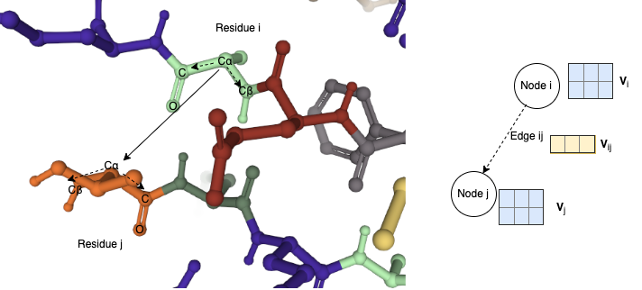Illustration of vector features on a protein geometric graph. The left panel depicts amino acid residues from a local neighborhood on a protein in 3D Euclidean space. Amino acid residues are colored by their types. Key atoms ($C$, $O$, $C\alpha$, $C\beta$) are labeled for two selected residues. Within residues, two vectors ($C\alpha - C\beta$ and $C\alpha - C$) are plotted in dashed arrows form the node feature \(\mathbf{V}_i \in \mathbb{R}^{2 \times 3}\). Between residue i and j, the vector $C\alpha_i - C\alpha_j$ can be used as the edge vector features $\mathbf{V}_{ij} \in \mathbb{R}^{1 \times 3}$. The right panel abstracts the protein geometric graph and their vector features.

Inherently interpretable by visualizing the learned vector field

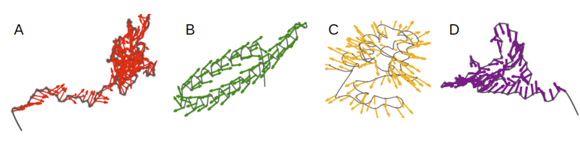
Because GVP-GNN learns and updates vector features on nodes and edges, it’s possible to visualize the learned vector features at the intermediate GVP-GNN layers. The set of learned vector features on a geometric graph actually resembles a vector field. We can try to interpret the learned vector field with some intuitions from physics. For instance, we can imagine the learned vector field represents force or velocity, although such interpretation needs to be rigorously investigated.

The authors visualized the learned node vector features on protein geometric graphs. We can clearly see the distinctive patterns on different protein graphs: contracting (A and D), rotating (B) expanding (C). It would be really interesting to study if those learned vector fields actually are correlated with intramolecular forces among the amino acid residues in the protein graphs.

In addition to looking at the resultant vector fields (analogous to feature maps in CNN), one should also analyze GVP’s kernels (\(\mathbf{W}_{\mu}\) and \(\mathbf{W}_{h}\)) because they are the counterpart to CNN’s kernels (aka filters), where lower level kernels learn to detect edge and texture and higher level kernels learn more complex images components such as animal eyes (think DeepDream/Inceptionism).

Applications of GVP-GNN within and beyond macro-molecules

Jing et al. demonstrated the application of their GVP-GNN to various supervised learning tasks on proteins represented as geometric graphs of amino acid residues. A natural next step is to model the protein geometric graphs at atomic level. With its expressiveness in geometric graphs, it would be interesting to see if high-resolution atomic graph representation of proteins improves various benchmarks in protein biology including protein design, and model quality assessment. Looking ahead, GVP-GNN has promising potential in improving protein structure prediction. For instance, in the AlphaFold2 framework (Jumper et al. 2021), invariant point attention (IPA) module is currently used to refine the high-resolution residue protein structure. Can GVP-GNN perform better than the IPA module on this task? Geometric graphs constructed from other macro-molecules like RNA and small molecules are immediate testbed for GVP-GNN, we also foresee broader applications in other domains.

Geospatial data as geometric graphs

In recent development of intelligent transportation systems (ITS), forecasting traffic speed, volume or the density of roads in traffic networks is fundamentally important. Considering the traffic network as a spatial-temporal graph, GNNs are ideally suited to traffic forecasting problems because of their ability to capture spatial dependency. A widely used application is the estimated times of arrival (ETAs) prediction in Google Map by DeepMind (Lange and Perez, 2020). However, current GNN solutions for these use cases only represent the data using regular graphs without geometric features. Traffic accident and anomaly prediction is a particularly challenging example: it involves accident records, geometric road structures, and meteorological conditions in addition to road networks. For example, the direct sunlight behind a steep hill or a sharp turn with no lane separation significantly increase the accident risk, and could be modeled in the GVP-GNN by considering geometric relations between road nodes and edges, i.e., encoding nodes with 3D vector features representing the geographic coordinates (latitude, longitude, and altitude). Jiang and Luo (2021) mentioned other use cases such as parking availability and lane occupancy forecasting that are likely to benefit from introducing geometric relations.

Another geospatial use case is the problem of collision-free navigation in multi-robot systems where the robots are restricted in observation and communication range. Positional relations between the robot fleet are crucial to the task. In Li et al. (2019), they jointly trained two networks: a CNN that extracts adequate features from local observations, and a GNN that learns to explicitly communicate these features among robots. GVP-GNN has the potential to determine what information is necessary and effectively communicate to facilitate efficient path planning.

Application in graph drawing

Graph drawing algorithms (aka network layout algorithms) are used to compute the 2D or 3D coordinates of nodes from a graph to preserve their local and global topological structures. They are commonly used for visualizing graphs and are closely related to some non-linear dimensionality reduction algorithms such as Laplacian Eigenmaps, which applies principal component analysis on the Laplacian matrix of the affinity graph constructed from the input data. Common graph drawing algorithms simulate physical forces among nodes and edges. For instance, the Fruchterman-Reingold algorithm is an iterative method that defines attractive and repulsive forces among nodes based on whether they are connected, with the objective of minimizing the energy of the system until equilibrium. Force-directed graph drawing algorithms are computationally expensive: cubic time to the number of nodes $\mathcal{O}(n^3)$. This is because the number of iterations is estimated to be $\mathcal{O}(n)$, and in every iteration, all pairs of nodes are visited and their mutual repulsive forces computed ($\mathcal{O}(n^2)$ complexity).

When we revisit the graph drawing problem, we notice that it can be formulated as a node-level task on a geometric graph: given a graph, we compute the coordinates of nodes ($\mathbf{V}_i \in \mathbb{R}^{1 \times d}$, where $d$ equals 2 or 3, for visualization in 2D or 3D, respectively) that minimize the energy function. GVP-GNN can be plugged in as a function approximator to solve this problem. The node vector features can be initialized randomly, just like in force-directed graph drawing algorithms where the positions of the nodes are initialized randomly. Graph drawing with GVP-GNN can reduce the time complexity of force-directed algorithms because each message passing epoch of GVP-GNN only costs $\mathcal{O}(m)$, where $m$ is the number of edges, which is guaranteed to be $m \leq n^2$.

Conclusion

In this post, we highlighted the novelties of GVP-GNN developed by Jing and colleagues, including the provable $E(3)$-invariance and equivariance, extension of the universal approximation guarantee, inherent interpretability by visualizing the learned vector features, and its SoTA performance on tasks related to protein structures.

More importantly, we analyzed how GVP-GNN fits into the Geometric Deep Learning blueprint and how it unifies two types of symmetries in geometric graphs. Through this post, we hope we inspire the readers with the breadth of under-utilized applications of geometric graphs and Euclidean equivariant GNNs: spanning from biochemical and geospatial data to network visualization and many more to follow!

References

• Justin Gilmer, Samuel S. Schoenholz, Patrick F. Riley, Oriol Vinyals and George E. Dahl (2017): “Neural Message Passing for Quantum Chemistry” arXiv:1704.01212
• Kristof T. Schütt, Pieter-Jan Kindermans, Huziel E. Sauceda, Stefan Chmiela, Alexandre Tkatchenko and Klaus-Robert Müller (2017): “SchNet: A continuous-filter convolutional neural network for modeling quantum interactions” arXiv:1706.08566
• Nathaniel Thomas, Tess Smidt, Steven Kearnes, Lusann Yang, Li Li, Kai Kohlhoff and Patrick Riley (2018): “Tensor field networks: Rotation- and translation-equivariant neural networks for 3D point clouds” arXiv:1802.08219
• Fabian B. Fuchs, Daniel E. Worrall, Volker Fischer and Max Welling (2020): “SE(3)-Transformers: 3D Roto-Translation Equivariant Attention Networks” arXiv:2006.10503
• Michael M. Bronstein, Joan Bruna, Taco Cohen and Petar Veličković (2021): “Geometric Deep Learning: Grids, Groups, Graphs, Geodesics, and Gauges” arXiv:2104.13478
• John Jumper et al. (2021) “Highly accurate protein structure prediction with AlphaFold” Nature doi.org/10.1038/s41586-021-03819-2
• Oliver Lange, Luis Perez (2020): “Traffic prediction with advanced Graph Neural Networks”
• Weiwei Jiang, Jiayun Luo (2021): “Graph Neural Network for Traffic Forecasting: A Survey” arXiv:2101.11174
• Qingbiao Li, Fernando Gama, Alejandro Ribeiro, Amanda Prorok (2019): “Graph Neural Networks for Decentralized Multi-Robot Path Planning” arXiv:1912.06095
• Andrew Y. Ng, Michael I. Jordan, Yair Weiss (2001): “On Spectral Clustering: Analysis and an algorithm”
• Thomas M. J. Fruchterman, Edward M. Reingold (1991), “Graph Drawing by Force-Directed Placement”, Software – Practice & Experience, Wiley, 21 (11): 1129–1164, doi:10.1002/spe.4380211102
• Yehuda Koren (2005): “Drawing graphs by eigenvectors: theory and practice”, Computers & Mathematics with Applications, 49 (11–12): 1867–1888, doi:10.1016/j.camwa.2004.08.015
• Markus Eiglsperger, Sándor Fekete, Gunnar Klau (2001): “Orthogonal graph drawing”, in Kaufmann, Michael; Wagner, Dorothea (eds.), Drawing Graphs, Lecture Notes in Computer Science, vol. 2025, Springer Berlin / Heidelberg, pp. 121–171, doi:10.1007/3-540-44969-8_6
• Michael Kaufmann, Dorothea Wagner(2001): “Drawing Graphs: Methods and Models”, Lecture Notes in Computer Science, vol. 2025, Springer-Verlag, doi:10.1007/3-540-44969-8