Symbolic Binding in Neural Networks through Factorized Memory Systems

25 Mar 2022 | symbolic memory binding Daigavane, Ameya; Khurana, Ansh; Bhardwaj, Shweta; Aggarwal, Gaurav

Our blog post describes the paper Emergent Symbols through Binding in External Memory that was published at ICLR 2021.

Introduction

Human intelligence is often described as ‘symbolic’ because we are able to take complex sensory inputs and map them to abstract concepts, represented by logical rules and symbols.

To illustrate this, consider the following scene with four objects of differing shape, size and color:

Many of us are able to quickly identify all of the objects in this scene. Once we do this, we can recognize certain logical relationships between the objects:

• The green cube is taller than the red cylinder.
• The red cylinder is taller than the yellow sphere.

Given just the last two statements however, we can quickly infer that “The green cube is taller than the yellow sphere”, even if we did not notice this when looking at the original image! We can formally denote this process of logical reasoning by the proposition:

\[(\text{G} > \text{R}) \text{ and } (\text{R} > \text{Y}) \implies (\text{G} > \text{Y}).\]

Here, we have assigned the height of the green cylinder to the symbolic variable $\text{G}$, expressed by the statement $G = \text{height}(\text{green cylinder})$, and so on. The assignment of a concrete value to an abstract symbol is called binding (or variable-binding).

Humans have an immense ability to understand abstract relationships and reason about them in a logical manner. This is due to our ability to reason using abstract symbols (such as $G$) without worrying about their concrete values (such as the exact height of the green cylinder).

However, such abstract reasoning has been difficult to emulate artificially; many state-of-the-art language generation models today struggle at simple logical tasks that even children excel at.

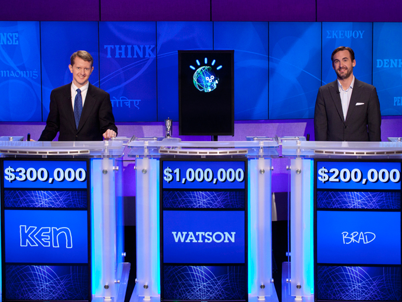
The drive to create intelligent systems that could perform some sort of logical reasoning is not recent. In the 1980s, research focused on symbolic systems (sometimes called classical AI) that tried to model knowledge as a vast body of logical statements that could then be queried over. These were wildly successful at the time: best illustrated by expert systems such as MYCIN and Dendral, and IBM’s Watson that won at ‘Jeopardy!’.

However, a major limitation of these systems was the need for well-defined structured inputs. In our CLEVR example above, they would need external supervision to identify the different objects and their properties in the scene. Thus, such ‘classical’ systems lacked the ability to infer structure from high-dimensional sensory observations of the world.

As a result, interest has gradually shifted to intelligent systems that can operate naturally on ‘raw’ high-dimensional data such as audio and video, exemplified by the rise of deep learning. The promise of deep learning is to do function approximation in a high-dimensional space, enabling predictive models that can operate on ‘raw’ data. While deep learning models have led to pivotal breakthroughs across multiple domains - computer vision, natural language processing, robotics, to name a few - the downside is that these models are effectively ‘black boxes’ with little insight into what exactly is being modelled.

The paper Emergent Symbols through Binding in External Memory that we will describe in this blog post shows that careful design choices can encourage neural networks to do symbolic reasoning, while still operating on high-dimensional inputs.

Symbolic Tasks

To understand how well machine learning models can perform abstract reasoning, the authors construct a set of $4$ increasingly difficult tasks:

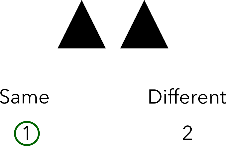
• Same-Different: Identify whether two images are the same or different from each other.

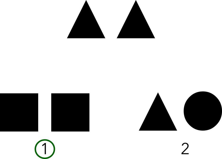
• Relational Match-To-Sample (RMTS): Given a source pair of images which have some relationship between them, identify which of two target pairs of images have the same relationship. Here, the authors considered the ‘same-different’ relationship: the source pair consists of either the same or different images.

• Distribution of Three: A row of three distinct images is provided. This row is permuted to form a second row of images, but the last image is removed. Identify which of four options was the removed image from the second row.

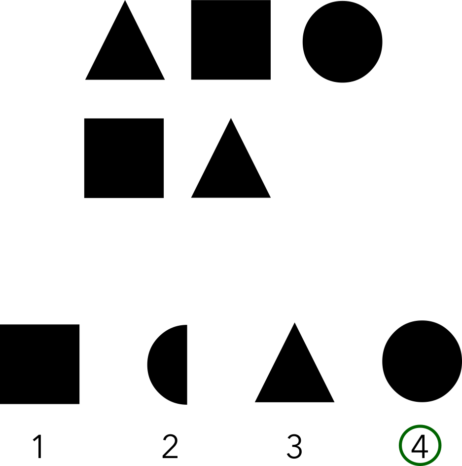
• Identity Rules: A row of images following a repetition rule (ABA, ABB, or AAA) is provided. A second row of images is provided, with the last image removed. Identify which of four options should be filled in the second row to follow the same repetition rule.

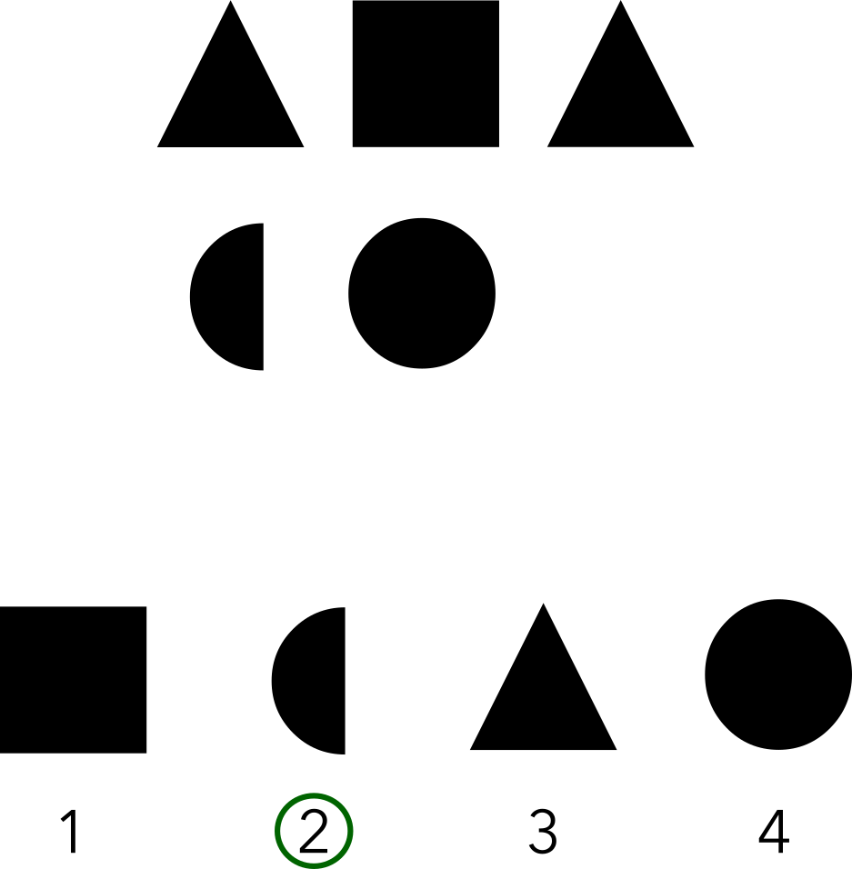
The authors create a pool of $100$ common symbols (eg. the triangle and square above). For each task, $m$ symbols are kept withheld, completely unseen during training. The remaining $100 - m$ symbols are used to generate example problems in the training set. To test generalization capabilities, the training set is limited to a size of $10000$ problems, which is much smaller than the total number of problems that can be created with these $100$ symbols.

Models Evaluated

Each instance of these tasks can be thought of as a sequence, where the individual input images and options are presented one timestep at a time. The final prediction (for example, a softmaxed probability over the four options) can be generated after the entire sequence is seen.

With this in mind, the overall setup that the authors consider consists of two stages:

• The Image Encoder $f_e$: Maps input images at each timestep to an embedding vector. Most of the experiments in the paper use a trainable convolutional neural network (CNN) for the image encoder, but there are additional experiments with a trainable multi-layer perceptron (MLP) and a fixed random CNN too.
• The Sequence Model $f_s$: Operates on the output of the image encoder to generate the final predictions. The authors consider multiple strong baselines for the sequence model here, described in the next subsections.

1. Emergent Symbol Binding Network

The Emergent Symbol Binding Network (ESBN) is one of the key contributions of this paper.

The ESBN consists of an LSTM controller with access to an external memory $M$. The external memory allows the LSTM controller to ‘remember’ what it has seen before. Further, the memory is factorized into a key component $M_k$ and a value component $M_v$. This memory supports only insertions: at each timestep, a single key-value pair is appended to the memory.

As a high level summary, the ESBN performs the following operations at every timestep t:

• Encode $x_t$ with the image encoder $f_e$ to get $z_t$.
• Compute the ‘read key’ $k_{r_t}$ using $z_t$.
• Use $k_{r_t}$ to update LSTM hidden state $h_{t}$.
• Compute the ‘write key’ $k_{w_t}$ using the LSTM.
• Write key $k_{w_t}$ to memory $M_k$ and value $z_t$ to memory $M_v$.

Below is an animated description of these operations:

For ease of exposition, we have chosen a different (but completely equivalent) order of operations here than the original paper.

We now describe exactly how the ‘read key’ and ‘write key’ are computed.

Computing the Read Key $k_{r_t}$

First, we compute weights $w$ over the values existing in $M_v$:

\[w = \text{softmax}(M_v \cdot z_t)\]

Compute confidence values $c$:

\[c = \sigma\left(\gamma (M_v \cdot z_t) + \beta \right)\]

where $\sigma$ is the sigmoid activation, so that each $c_i$ is bounded between $0$ and $1$. $\gamma$ and $\beta$ are learnt gain and bias parameters. The confidence values are useful to indicate how much of a match is present between the current encoded symbol $z_t$ and the values already seen in memory. Unlike the weights $w$, the confidence values do not have to sum up to $1$. The confidence values especially help for the Same-Different and RMTS tasks, where the ability to directly answer whether a particular symbol has been seen before is particularly useful.

We concatenate the confidence values $c_i$ to the keys $M_{k_{i}}$, weight them by the attention weights $w_i$, sum them up, and pass them through the gated mechanism $g_{t - 1}$ to get the ‘read key’ $k_{r_t}$:

\[k_{r_t} = g_{t - 1}\left(\sum_{i = 1}^{t - 1} w_i \left(M_{k_{i}} \parallel c_i\right)\right)\]

Updating the LSTM Hidden State

We use the just-computed ‘read key’ $k_{r_t}$ to update the LSTM’s hidden state:

\[h_t = \text{LSTM}(h_{t - 1}, k_{r_t})\]

Computing the Write Key $k_{w_t}$

We use the LSTM’s update hidden state $h_t$ to compute the next ‘write key’ $k_{w_t}$, as well as the gated mechanism $g_t$ for the next timestep and output $y_t$:

\[\begin{aligned} k_{w_t} &= \text{ReLU}(\text{Linear}(h_t)) \\ g_t &= \sigma(\text{Linear}(h_t)) \\ y_t &= \sigma_{\text{pred}}(\text{Linear}(h_t)) \\ \end{aligned}\]

where $\sigma_{\text{pred}}$ is either the sigmoid activation or the softmax activation, depending on the number of options present.

This key $k_{w_t}$ is now concatenated to the memory $M_k$:

\[M_{k} \leftarrow M_{k} \parallel k_{w_t}\]

and the associated value $z_t$ representing the encoded image at the current timestep is concatenated to the memory $M_v$:

\[M_{v} \leftarrow M_{v} \parallel z_t\]

Note that the LSTM controller never operates directly on the encoded image representations ${z_t}$. Thus, the keys computed by the LSTM controller can be thought of as abstract ‘symbolic’ representations of the input seen so far. In a later section, we will justify why we can call these representations ‘symbolic’ by a visual analysis for the different tasks.

The paper compares the performance of the ESBN against some popular baselines. To understand how the ESBN differs from these baseline models, we now describe their working in detail.

2. Neural Turing Machines (NTM)

The Neural Turing Machine couples a recurrent neural networks with an external memory. This external memory is accessed by an attention-based mechanism. The memory matrix in the NTM is an updatable fixed-size look-up table unlike the ESBN where entries are concatenated to the memory at each timestep and cannot be overwritten.

As another point of comparison, the NTM uses multiple separate read and write heads, thus enabling parallel reads and writes to the memory.

Each read head produces a weighting $w_t$ over the memory indices, and the value $r_t$ read from the memory is simply a convex combination of the memory values with these weights:

\[r_t = \sum_i w_t(i) M(i)\]

Each write head generates a weighting $w_t$ over the memory indices, a common erase vector $e_t$ and a common add vector $a_t$. The index $i$ in the memory is then updated as:

\[M(i) \leftarrow M(i) \odot [1 − w_t(i)e_t] + w_t(i)a_t\]

where $\odot$ indicates element-wise multiplication.

To compute these weightings $w_t$, the NTM makes use of both content-based as well as location based addressing. In particular, each read head generates a read key vector $k_t$ and a key strength $\beta_t$ to compute the content-based weights $w^{(c)}_t$ as:

\[w^{(c)}_t = \text{softmax}\left(\beta_t \cdot \text{sim}(k_t, M_t(i))\right)\]

where $\text{sim}$ is the cosine similarity measure. The read head then generates a gate value $g_t \in (0, 1)$ to weigh the content-based weights $w^{(c)}_t$ relative to the weights at the previous timestep:

\[w^{(g)}_t = g_t w^{(c)}_t + (1 - g_t)w_{t - 1}\]

Then, to allow for rotational shifts of the memory, the read head generates a softmaxed shift vector $s_t$, which is then used to aggregate weights across neighbouring positions in the memory:

\[w^{(r)}_t(i) = \sum_{j = 1}^N w^{(g)}_t(j) \cdot s_t((i − j) \ \text{mod} \ N)\]

The final weights $w_t$ are obtained by sharpening these weights to avoid ‘blurring’ of the same content across multiple memory indices. This is controlled by another scalar $\gamma_t$ emitted by the read head:

\[w_t = \text{softmax}\left(\left(w^{(r)}_t\right)^{\gamma_t}\right)\]

In conclusion, the NTM’s memory addressing mechanism is quite sophisticated compared to that of the ESBN. Training such a mechanism can also be quite difficult, however. A key difference is the explicit factorization of ESBN’s memory between the image embeddings (what it perceives) and the corresponding ‘symbolic’ representations.

3. Metalearned Neural Memory (MNM)

The external memory used in both the ESBN and the NTM are simple in the way they are implemented as a large look-up table of values. An alternative approach is to model memory itself as a function, as explored in Metalearned Neural Memory.

To be precise, the output from the memory is a function $M$ of the input query. The key idea is to parametrize the memory $M$ by a neural network. At every timestep $t$, an LSTM controller outputs three quantities:

• The read-in key $k_{r_t}$
• The write-in key $k_{w_t}$
• The values $v_{w_t}$

The read-out keys $v_{r_t}$ are then computed via a forward pass of the memory $M_t$:

\[v_{r_t} = M_t(k_{r_{t}})\]

For the write-out keys $\hat{v}_{w_t}$, the process is similar, but uses the memory parameters from the previous timestep:

\[\hat{v}_{w_t} = M_{t - 1}(k_{w_{t}})\]

The parameters of the memory $M$ are optimized to encourage binding by minimizing the distance between the values $v_{w_t}$ and the write-out keys $\hat{v}_{w_t}$.

In contrast to the ESBN where the LSTM controller only controls what is written to the memory, the LSTM controller in the MNM generates two sets of keys, $k_{r_t}$ for reading and $k_{w_t}$ for writing to the memory. To recall, in the ESBN, the key being read from the memory is computed using the encoded image at the current timestep.

4. Transformers

Transformers have become extremely popular in sequence modelling problems. Compared to the three models just discussed which process inputs one at a time, the Transformer processes the entire sequence at once to generate a prediction. The core of the Transformer is the self-attention block, described below.

First, we linearly project the encoded image $z_t$ to a query $q_t$, a key $k_t$ and a value $v_t$:

\[q_t = W_q \cdot z_t \\ k_t = W_k \cdot z_t \\ v_t = W_v \cdot z_t\]

Then, we compute the attention weights $w_t \in \mathbb{R}^T$ for each timestep:

\[w_t = \text{softmax}\left(q_t \cdot k_i\right)\]

and then use these weights to combine the values, giving us a new embedding $z’_t$ for each timestep:

\[z'_t = \sum_{i = 1}^T w_{t_i} v_i\]

These embeddings ${z’_t}$ are passed through a shared MLP, averaged and provided as input to another MLP to generate a final prediction.

5. Relation Networks

The Relation Network is a general architecture that explicitly models pairwise relations between instances. In particular, given the sequence $\{z_t\}$ of encoded images, the Relation Network $\text{RN}$ computes:

\[\text{RN}(\{z_t\}) = f\left(\sum_{t, t'} g(z_t, z_{t'})\right)\]

where $f$ and $g$ are parametrized by neural networks.

The Relation Network can be seen as an extension of the Deep Sets architecture to allow for pair-wise relations:

\[\text{DS}(\{z_t\}) = f\left(\sum_{t} g(z_t)\right)\]

Like Deep Sets, the Relation Network is invariant to the ordering of the images in the input. To give the Relation Network information about the exact positions of the images in the input, every embedding $z_t$ was appended with the integer $t$ as a ‘temporal tag’ feature.

This positional information is essential when considering the Distribution of Three and Identity Rules tasks. The Relation Network however cannot model ternary relations (that is, relations between three objects $z_t, z_{t’}, z_{t’’}$), which explains its poor performance on these tasks. A variant of the Relation Network called the Temporal Relational Network that can explicitly model ternary relations performed better on these tasks.

6. PrediNet

Similar to the Relation Network, the PrediNet takes a relation-oriented modelling approach, but using self-attention blocks, similar to the Transformer.

The PrediNet consists of multiple heads, the outputs of which are simply concatenated at the end. For clarity, here we describe the operation of a PrediNet with only one head.

Given the sequence of embeddings $\{z_t\}$ as a matrix $L$ of leading dimension $T$, PrediNet first flattens $L$. Then, it computes two sets of query vectors $Q_1$ and $Q_2$, and a key matrix $K$:

\[\begin{aligned} Q_1 &= \text{flatten}(L)W_{Q1} \\ Q_2 &= \text{flatten}(L)W_{Q2} \\ K &= LW_{K} \\ \end{aligned}\]

The query vectors $Q_1$ and $Q_2$ are specific to each head, while the key matrix $K$ is shared across heads.

Each entry in $K$ is now queried against both $Q_1$ and $Q_2$, and the result is softmaxed to give weight vectors $w_1$ and $w_2$, each of dimension $T$. Informally, these weight vectors indicate how much each of the $T$ objects match with the query vectors $Q_1$ and $Q_2$.

\[\begin{aligned} w_1 &= \text{softmax}(Q_1K^T) \\ w_2 &= \text{softmax}(Q_2K^T) \\ \end{aligned}\]

Then, these weight vectors are used to compute two representations $E_1$ and $E_2$ of the entire sequence as:

\[\begin{aligned} E_1 &= w_1L \\ E_2 &= w_2L \\ \end{aligned}\]

Then, the difference between these representations is computed, and mapped to a $j$ dimensional vector by multiplying with $W_S$.

\[D = (E_1 - E_2) W_S\]

This vector $D$ is passed to an MLP to generate the final predictions.

Temporal Context Normalization

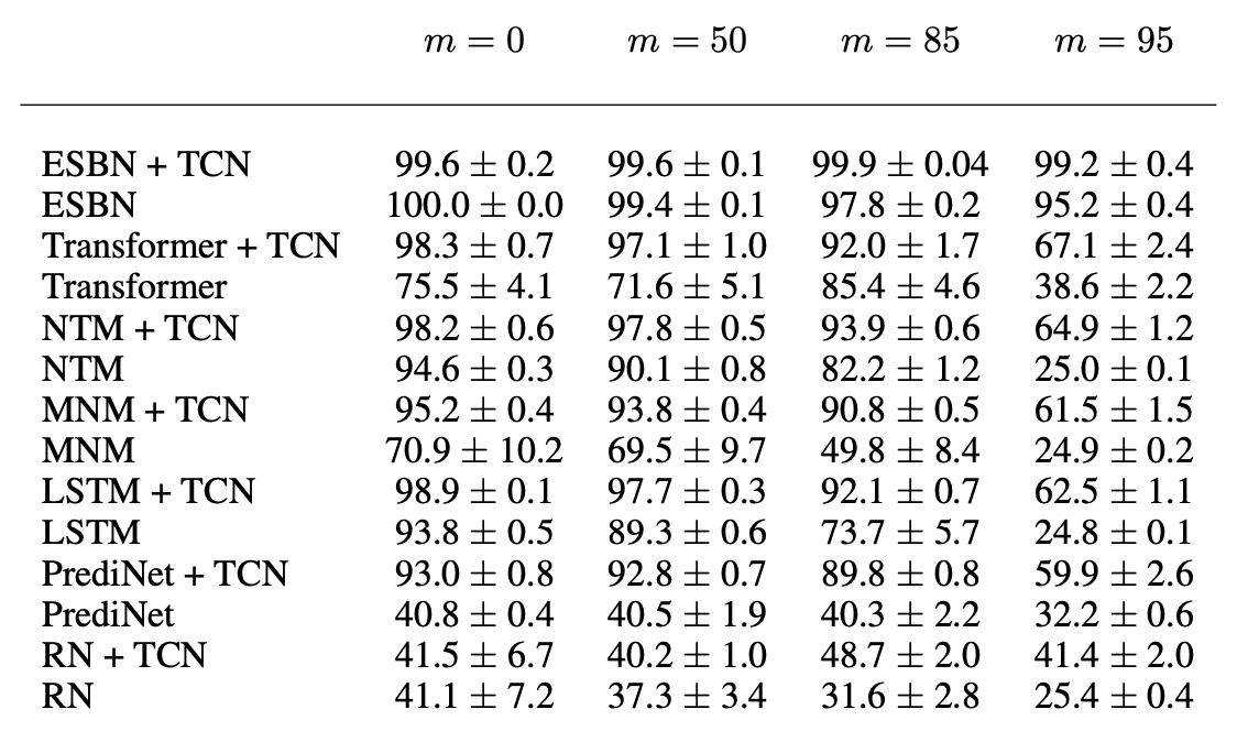
The authors found that normalization across the timestep axis, termed Temporal Context Normalization (TCN), helped the performance of all models significantly. In the table below, $m$ refers to the number of withheld symbols (out of $100$) that are not observed during training.

Consider a batch $Z$ consisting of $B$ sequences of encoded images, each of length $T$, where each encoded image has $K$ features. Then, by $Z_{itk}$, we mean the $k$th feature of $z_t$ where $\{z_t\}_{t = 1}^T$ is the $i$th sequence in the batch. Then, TCN performs the following normalization:

\[\begin{aligned} \mu_{ik} &= \frac{1}{T}\sum_{t = 1}^{T} Z_{itk} \\ \sigma_{ik} &= \sqrt{\frac{1}{T}\sum_{t = 1}^{T} (Z_{itk} - \mu_{ik})^2 + \epsilon} \\ Z'_{itk} &= \frac{Z_{itk} - \mu_{ik}}{\sigma_{ik}} \\ \end{aligned}\]

where $\epsilon$ is a small positive value to avoid division by zero. Thus, TCN is the analogue of batch normalization, but applied to the timestep axis, instead of the batch axis.

In this work, TCN is applied to the full sequence of $\{z_t\}$ obtained from the image encoder $f_e$. The normalized sequence $\{z’_t\}$ is then fed in to the sequence model $f_s$.

Visualizing ESBN’s Symbolic Representations

To understand if ESBN’s representations are indeed instance independent, and capture the task dependent properties for predicting the correct answers, we visualize the learnt representations in the memory for all four symbolic tasks studied in the paper. The keys written to the memory ($k_{w_t}$) are the outputs of the ESBN network, which describe the information ESBN stores for future at current time step ($t$). The keys retrieved from the memory ($k_{r_t}$) represent the input to the LSTM, and thus decide the output for the current time step ($t$). We plot the first three principal components of variations in all plots, which cover more than $90\%$ variation in the representations for each of the four tasks.

Visualization the Evolution of Representations

As mentioned above, the ‘write’ keys $k_w$ computed by the ESBN can be thought of as symbolic representations of the encoded image seen at each time step. We train the ESBN model with the provided hyper-parameters for each of the symbolic tasks to generate these representations. All experiments are performed with a train set of $5$ symbols, and thus, a test set of $95$ unseen symbols.

Below, we illustrate how the key representations evolve during training, starting from their values at initialization for the first 100 training steps. The learnt key representations ($k_w$) across different time step are shown using different colors. We observe that the keys computed by ESBN model seem to be independent of the actual image being encoded.

Same-Difference Task: Evolution During Training

For the Same-Different task, we find that the ESBN learns to separate the two timestep representations without any dependence on the actual symbol being encoded.

RMTS Task: Evolution During Training

The ESBN only requires a few epochs to converge for the RMTS task. The variance of key representations increases with $t$, indicating some level of uncertainty. A possible explanation is that once the first option pair at $t = 3, 4$ has been seen, the ESBN model can technically already guess the right answer, without actually seeing what the second option pair is at $t = 5, 6$, since exactly one of the option pairs is always correct. This means the network might not need to exactly localize the representations of the second option pair at $t = 5, 6$ to obtain good performance.

Distribution of Three Task: Evolution During Training

Similar to the RMTS task, the ESBN requires only a few epochs to converge for the Distribution of Three task. For clarity, we plot the key representations only corresponding to the questions, not the options. The option time steps are very diffused since only one of the options is correct and the other options map to ‘nonsensical’ symbols. We see that the key representations for each time step cluster well.

Identity Rules Task: Evolution During Training

In the Identity-Rules task, the representations do not cluster as well as in the other tasks, but there is still a clear structure. This is because of the added complexity here where the ESBN has to identify one of three repetition rules from the question. As above, we plot the key representations only corresponding to the questions, not the options.

For all tasks, the keys written at the first two time steps ($t=1,2$) are tightly clustered at one location for all training examples. From the third time step onwards, the encoded key is task dependent. Tight clustering of key representations for a given time step represent the capabality of ESBN to learn task-dependent symbolic representations across different examples for the given task.

The Generalizability of ESBN Representations

In the following subsections, we compare ESBN representations for train and test instances, across the four different tasks. Overall, we find that there is significant overlap in the structure of the train and test representations, even though the test symbols are completely unseen during training.

This explains why the ESBN model is able to generalize to near-perfect accuracy on all tasks unlike any of the other baselines, even when the ESBN has observed only a small subset of symbols during training.

Same-Different Task: Generalization

In this plot we show the keys written by the ESBN network ($k_w$) at $t=1$, and how it compares to the key that the network reads after seeing the second input at $t=2$. The LSTM predicts whether the input at $t=2$ is same as or different from the input at $t=1$ using the input $k_{r_2}$ and the hidden state $h_1$. The figure shows how representations of $k_{r_2}$ differ based on whether the example is Same or Different, showing how ESBN creates a decision boundary for these two cases. Further, the strong clustering for these two cases show that ESBN learns instance invariant representations as claimed in the paper. This generalisation is observed for both test and train examples, and the representations align closely.

RMTS Task: Generalization

For the RMTS task, we plot the representations for $k_{r}$ for $t= 3$ and $4$ denoting the two possible cases for each example. The output of ESBN model would depend on whether the inputs at $t= 3$ and $4$ follow the same relationship as inputs at $t= 1$ and $2$. This can be observed in the segregation between same relation (green and orange) and different relation (purple and sky blue) $k_r$ representations. For the same relation case, the test representations align well with the train representations. However, when there is a different relation, the test representations seem to interpolate between the clusters formed by the train representations.

Distribution of Three Task: Generalization

For the Distribution of Three task, the first three inputs uniquely determine the symbols for the next three time steps. We plot the retrieved representations ($k_r$) for the first match of the corresponding input at $t = $ 1, 2 and 3. In the plot, we observe that the test representation closely matches with the train representation within the expected range of the training examples. However, there are lot of outlier data points in the test representation. The generalisation of performance on the test distribution is not perfect, and the representations do not align well with the train distribution. In the appendix of the paper, the representations for the test distribution are shown only in range of the train representation. When observed in this range, the train and test representations are well aligned. However, there are some outlier test instances which outside the train representations range showing that the alignment is not perfect.

Identity-Rules Task: Generalization

For the Identity-Rules task, we plot the $k_w$ representations for the time steps corresponding to the question, and see how the keys $k_r$ read for the different correct differ. The repetition rules in the Identity Rule task are of three types - ABA, ABB, or AAA. Based on the repetition rule, and the sequence of inputs seen so far, there is high variation in the representations. For the four option time steps, we plot the representations for each correct or incorrect option separately. Since an incorrect option in one example, (say symbol B if the rule is ABA) could be the correct option for another example (symbol B would be the correct answer if the rule is ABB), there is high variation for both the incorrect and correct option time steps. Further, the representations are intermixed. For the Identity-Rules task, the train and test representations align closely.

Based on our analysis of the retrieved and written representations encoded by ESBN, we can infer that the model is indeed able to abstract symbol-like representations (such as ‘first image’, ‘second image’, ‘same image as second’) which are independent of the identity of images. Even under the strong setting of $95$ heldout symbols, the model generalises extremely well (albeit not perfectly) on the test set.

Open Questions and Conclusion

The ideas in this paper raise some important questions:

• The datasets investigated here are rather simple. Can such factorized memory systems solve more complex visual tasks, such as answering questions from the CLEVR dataset?
• Can we achieve similar performance without requiring linear $\Theta(T)$ memory? Improvements here will enable the wider use of augmented memory systems, especially for problems that require larger temporal context.
• Can factorized memory allow for the joint processing of multi-modal inputs, where the use of symbolic representations would enable reasoning across modalities such as text and video?
• There is a certain appeal in simplicity, but would ESBN benefit from more complex memory addressing mechanisms beyond simple dot-products, such as those found in the NTM?

In conclusion, we have described the motivation and working of the ESBN in great detail, compared its design choices to strong baselines, and performed a qualitative validation of the generalization claims from the original paper. We believe the community will benefit from the clear exposition of the valuable ideas in this paper.

Contributions Statement

Ameya Daigavane and Ansh Khurana contributed equally to the creation of this blog post. Ameya wrote most of the blog post and helped improve the animation of the ESBN model that Ansh initially created. Ansh trained the models and generated all of the interactive visualizations in this blog post. Shweta Bharadwaj and Gaurav Aggarwal helped brainstorm the overall structure and high-level content of the blog post.