On Dyadic Fairness: Exploring and Mitigating Bias in Graph Connections
25 Mar 2022 | graphs fairness representation-learningThis blog post discusses the ICLR 2021 paper “On Dyadic Fairness: Exploring and Mitigating Bias in Graph Connections” by Li et al., highlighting the importance of its theoretical results while critically examining the notions and applications of dyadic fairness presented. This blog post assumes basic familiarity with graph representation learning using message-passing GNNs and fairness based on observed characteristics. The images in this blog post are equipped with alernative text.
Motivation
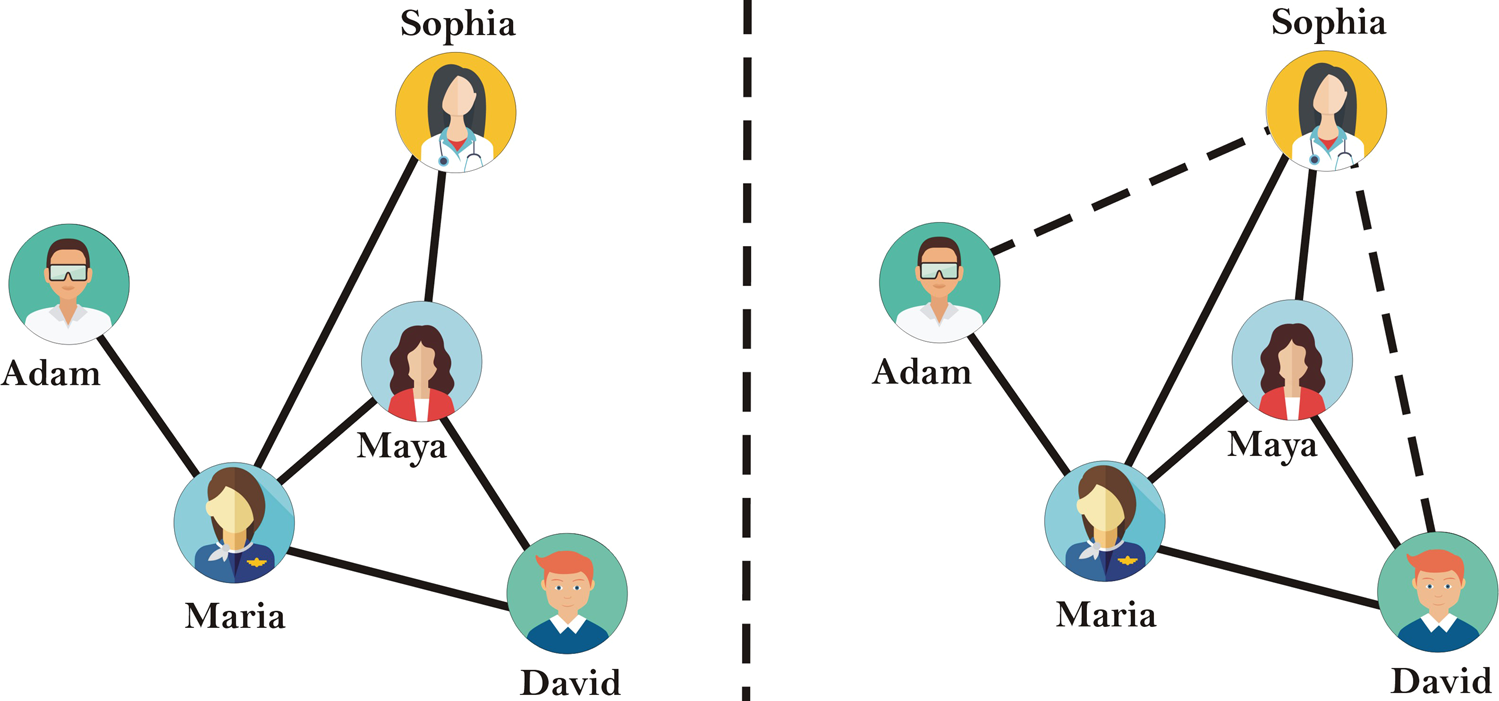
Link prediction is the task of predicting unobserved connections between nodes in a graph. For example, as shown in the social network in Figure 1, a link prediction algorithm may leverage the observed edges (solid lines) to predict that the node representing Sophia is also connected to the nodes representing Adam and David (dashed lines).
Link prediction is ubiquitous, with applications ranging from predicting interactions between protein molecules to predicting whether a paper in a citation network should cite another paper. Furthermore, social media sites may use link prediction as part of viral marketing to show ads to users who are predicted to be connected to other users who have interacted with the ads, because the users are assumed to be similar.
However, ads can influence users’ actions, and if a link prediction algorithm is tainted by social biases or exhibits disparate performance for different groups, this can have negative societal consequences. For instance, a social media site may only spread ads for STEM jobs within overrepresented groups like white men, rather than to women and gender minorities of color, because the site’s link prediction algorithm disproportionately predicts connections between members of overrepresented groups, and not between members of different groups. This can reduce job applications from marginalized communities, exacerbating already-existing disparities and reducing diverse perspectives in STEM.
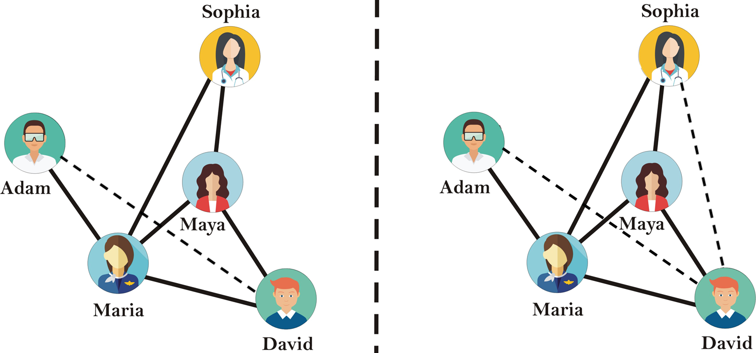
In the running social network example, suppose Sophia is a woman and that Adam and David are men. Furthermore, suppose David interacts with an ad for a software engineering position. In Figure 2, the left panel illustrates a binary gender-biased link prediction algorithm that only predicts a connection between David and Adam, and not between David and Sophia; this would result in only Adam and not Sophia seeing the software engineering ad. In contrast, the right panel illustrates a link prediction algorithm that predicts a connection between David and Adam and between David and Sophia. This algorithm satisfies what is called dyadic fairness (with respect to binary gender), as it predicts an equal rate of man-woman and man-man/woman-woman links. This could have a lower likelihood of amplifying binary gender disparities.
While I have constructed the example above, the authors of the paper “On Dyadic Fairness: Exploring and Mitigating Bias in Graph Connections” provide two other applications of dyadically-fair link prediction:
- delivering “unbiased” recommendations (i.e. recommendations that are independent of sensitive attributes like religion or ethnicity) of other users to friend, follow, or connect with on a social media site
- recommending diverse news sources to users, independent of their political affiliation
While polarization is a problem online, these applications of dyadically-fair link prediction could be problematic. Many marginalized communities (e.g. LGBTQIA+ folks; Black, Latine, and Indigenous individuals; etc.) create and rely on the sanctity of safe spaces online. Thus, recommending users or news sources that are hostile (e.g. promote homophobic, racist, or sexist content) can result in severe psychological harm and a violation of privacy. Furthermore, many individuals in these communities, because they feel isolated in real life, actually yearn to find other users online who share their identity, to which dyadic fairness is antithetical. In these cases, dyadic fairness doesn’t distribute justice.
High-Level Idea
The paper “On Dyadic Fairness: Exploring and Mitigating Bias in Graph Connections” contributes the following:
- mathematical formalizations of dyadic fairness
- a theoretical analysis of the relationship between the dyadic fairness of a graph convolutional network (GCN) and graph structure
- based on the analysis, an algorithm FairAdj that jointly optimizes the utility of link prediction and dyadic fairness of a GNN
Formalizations of Dyadic Fairness
Suppose we have an undirected, (possibly) weighted homogeneous graph $ G = (V, E) $, consisting of a fixed set of nodes $V$ and fixed set of edges $E$. Furthermore, assume that every node in $ V $ has a binary sensitive attribute, that is, it belongs to one of two sensitive groups.
To prevent notation overload upfront, I will present one mathematical formalization of dyadic fairness first and then dissect the notation. This formalization is based on Independence (also known as demographic parity or statistical parity) from the observational group fairness literature.
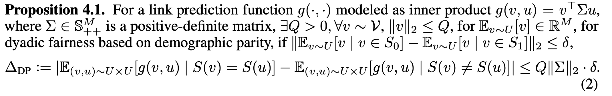
![Definition 3.1 from the paper. A link prediction algorithm satisfy [sic] dyadic fairness if the predictive score satisfy [sic] the distribution of the predictive score of a link between nodes u and v given that u and v belong to the same sensitive group equals the distribution of the predictive score of a link between u and v given that u and v do not belong to the same sensitive group.](https://iclr-blog-track.github.io/public/images/2022-03-25-dyadic-fairness/dyadic_fairness.png)
In Definition 3.1, $ g $ is the link prediction algorithm. It takes as input the representations of two nodes, which we will denote as $u$ and $v$, and outputs a predictive score representing the likelihood of a connection between $u$ and $v$. $ S $ is a function that takes as input a node $ i $ and outputs the sensitive group membership of $i$. For instance, in the running social network example, $ S(Sophia) = woman $.
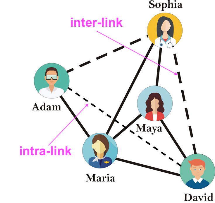
We define intra-links as edges connecting nodes belonging to the same sensitive group, and similarly, inter-links as edges connecting nodes belonging to different sensitive groups. As shown in Figure 4, $(David, Adam)$ is an intra-link, while $(David, Sophia)$ is an inter-link.
Then, we can see that this formalization of dyadic fairness simply requires that our link prediction algorithm predicts intra-links and inter-links at the same rate from the set of candidate links, i.e. $g(u, v) \bot S(u) = S(v)$.
The authors do empirically explore other formalizations of dyadic fairness based on Separation, i.e. $ g(u, v) \bot S(u) = S(v) | (u, v) \in E$:
- the disparity in predictive score between intra-links and inter-links for only positive links, i.e. $ Pr(g(u, v) | S(u) = S(v), (u, v) \in E) = Pr(g(u, v) | S(u) \neq S(v), (u, v) \in E) $
- the disparity in predictive score between intra-links and inter-links for only negative links, i.e. $ Pr(g(u, v) | S(u) = S(v), (u, v) \notin E) = Pr(g(u, v) | S(u) \neq S(v), (u, v) \notin E) $
- the maximum difference in the true negative rate (over all possible thresholds on the predictive score) between intra-links and inter-links
- the maximum difference in the false negative rate (over all possible thresholds on the predictive score) between intra-links and inter-links
It appears that the authors don’t explore possible formalizations of dyadic fairness based on Sufficiency: $ Pr((u, v) \in E | S(u) = S(v), g(u, v)) = Pr((u, v) \in E | S(u) \neq S(v), g(u, v)) $. Succinctly, Sufficiency can be expressed as $ (u, v) \in E \bot S(u) = S(v) | g(u, v) $. At a high level, Sufficiency posits that the predictive score “subsumes” the type of link (intra-link or inter-link) for link prediction, and the predictive score satistifies Sufficiency when links’ existence and type are “clear from context” (Barocas et al., 2019). Sufficiency could be an area for further exploration.
Interestingly, the formalizations of dyadic fairness based on Independence, Separation, and Sufficiency are mutually-exclusive except in degenerate cases (for the proof of this, consult Barocas et al., 2019).
Furthermore, each notion of fairness has its own politics and limitations. While Independence may seem desirable because it ensures that links are predicted independently of (possibly irrelevant) sensitive attributes, it can also have undesirable properties. For instance, a social network may have significantly more training examples of intra-links than inter-links, which could cause a learned link predictor to have a lower error rate for intra-links than inter-links. To be concrete, suppose this link predictor accurately predicts intra-links at a rate $p$ and simultaneously randomly predicts inter-links at a rate $p$ from candidate links. This link predictor satisfies Independence, but has wildly different error rates on intra-links and inter-links. Additionally, Independence does not consider associations between the existence of a link (the target variable) and whether it’s an intra-link or inter-link. In contrast, Separation and Sufficiency “accommodate” associations between the existence of a link and if it’s an intra-link or inter-link.
Moreover, all of Independence, Separation, and Sufficiency are limited in that they are based on observed attributes. Causality is emerging a lens through which fairness can be observed under intervention. However, all of the aforementioned methods and criteria assume that sensitive attributes are:
- known, which is often not the case due to privacy laws and the dangers involved in disclosing certain sensitive attributes (e.g. disability, queerness, etc.);
- measurable, which is almost never true (e.g. gender);
- discrete, which reinforces hegemonic, colonial categorizations (e.g. race and ethnicity options on the US census, the gender binary, etc.);
- static, which is problematic given that one’s identity can change over time (e.g. genderfluidity).
Furthermore, observational fairness neglects that some communities face complex, intersecting vectors of marginality that preclude their presence in the very data observed for fairness. Additionally, Independence, Separation, and Sufficiency, due to their quantitative nature and focus on parity, don’t capture notions of fairness based in distributive justice and representational justice (Jacobs and Wallach, 2021). Moreover, these criteria ignore historical and social context, and thus cannot “accommodate reparative interventions” to remedy past inequity (Cooper and Abrams, 2021).
These limitations could motivate future work in the areas of fair graph machine learning without access to sensitive attributes and with human-in-the-loop approaches to including fluid identities that defy categorization, as well as rethinking how fairness is operationalized more broadly in machine learning.
How does graph structure affect dyadic fairness?
In this section, we only consider the formalization of dyadic fairness in Definition 3.1, i.e. based on Independence. Suppose we have two sensitive groups $S_0$ and $S_1$. Furthermore, let $U$ be the uniform distribution over all the nodes in $V$ and $M$ be the dimension of node representations.
Let’s dissect what Proposition 4.1 means! Proposition 4.1 makes the assumption that our link prediction function $g$ is modeled as an inner product of the two input node representations. In this case, we can show that $\Delta_{DP}$, the disparity in the expected predictive score of intra-links and expected predictive score of inter-links, is bounded by a constant times $\delta$, the disparity in the expected representation of nodes in $S_0$ and expected representation of nodes in $S_1$. Why is this cool? It implies that a low $\delta$ is a sufficient condition for a low $\Delta_{DP}$.
Now we need to investigate how a graph neural network (GNN) affects $\delta$! As usual, I will present Theorem 4.1 and then dissect the notation.
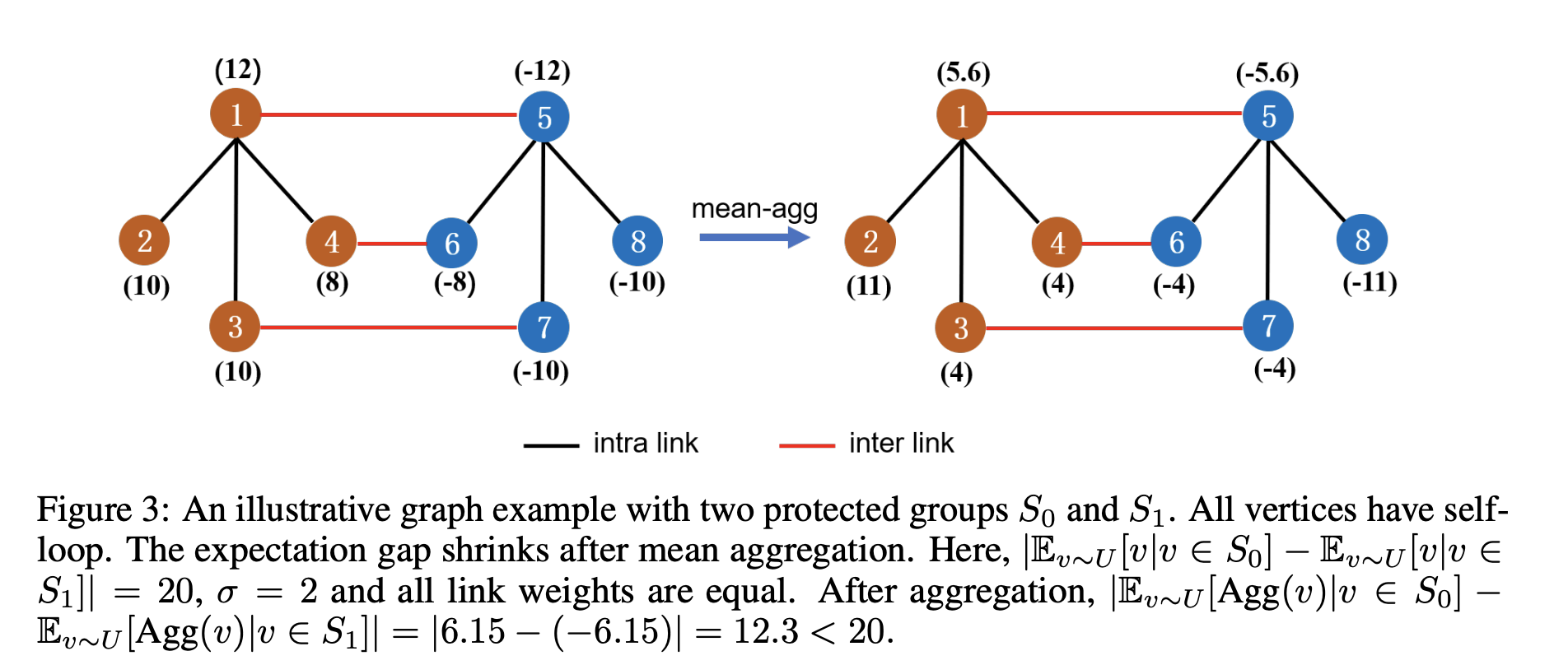
Theorem 4.1 looks at $\Delta_{DP}^{Aggr}$, the disparity in the expected representation of nodes in $S_0$ and expected representation of nodes in $S_1$ after one mean-aggregation over the graph. A mean-aggregation uses the graph filter $D^{-1} A$, where $A$ is the graph’s adjacency matrix with self-loops and $D$ is the diagonal degree matrix corresponding to $A$. However, many other graph filters are used in a variety of message-passing algorithms:
- $D^{-\frac{1}{2}} A D^{-\frac{1}{2}}$, which is the symmetric reduced adjacency matrix used in Graph Convolutional Networks (GCNs);
- $A D^{-1}$, which is the random walk matrix used in belief propagation and label propagation;
- $softmax(\frac{(Q X)^T (K X)}{\sqrt{d_k}})$, which is the scaled dot product attention matrix used in Transformers
Even an iteration of the Value Iteration algorithm for Markov Decision Processes can be reframed as applying a graph filter to a graph containing nodes representing states and actions and edges representing transitions! (To learn more about this, consult Lee, 2021.) The beauty of the proof of Theorem 4.1 is that, since aggregation is a central operation in every message-passing algorithm, the general procedure used in the proof can be followed to analyze representation disparities between sensitive groups in label propagation, Transformers, etc.
Back to dissecting Theorem 4.1! We will only look at the upper bound on $\Delta_{DP}^{Aggr}$. $\lVert \mu_0 - \mu_1 \rVert_2$ is the disparity in the expected representation of nodes in $S_0$ and expected representation of nodes in $S_1$ prior to the mean-aggregation over the graph. $\sigma$ is the maximal deviation of node representations, i.e. $\forall v \in S_0, \lVert v - \mu_0 \rVert_\infty \leq \sigma$ and $\forall v \in S_1, \lVert v - \mu_1 \rVert_\infty \leq \sigma$. Hence, we can see that $\alpha_{max}$ functions as a contraction coefficient on the representation disparity between the sensitive groups and $2 \sqrt{M} \sigma$ serves as a sort of error term on the contraction. $\alpha_{max}$ is regulated by the total weight of inter-links $d_w$ (relative to the maximum degree $D_{max}$ of nodes), as well as the number of nodes in each sensitive group incident to inter-links $\lvert \widetilde{S_0} \rvert$ and $\lvert \widetilde{S_1} \rvert$ (relative to the number of nodes in the groups $\lvert S_0 \rvert$ and $\lvert S_1 \rvert$).
$\alpha_{max}$ must be less than 1 for the mean-aggregation to reduce the disparity in expected representations; this is not the case for only a few graph families, e.g. complete bipartite graphs. The authors provide an excellent analysis characterizing various graphs and their corresponding $\alpha_{max}$ in Section B of the paper’s appendix, e.g. Figure 3 below.
As future work, it would be interesting to explore how the contraction coefficient $\alpha_{max}$ varies for different message-passing algorithms. It would also be exciting to investigate how this analysis changes for graphs that are heterophilic rather than homophilic, or have heterogeneous links.
Corollary 4.1 incorporates the learned parameters of a GCN into the bound on the disparity in expected representations between sensitive groups, but I will not cover the corollary in this blog post.
FairAdj
FairAdj is based on the idea that since a low $\delta$ is a sufficient condition for a low $\Delta_{DP}$, and the bound on $\delta$ is affected by $\alpha_{max}$, which is in turn affected by edge weights and the graph’s structure, we can modify the graph’s adjacency matrix to improve the fairness of an inner-product link prediction algorithm based on representations learned by a GNN.
The authors propose a simple, yet effective solution of alternating between training the GNN and optimizing the graph’s adjacency matrix for dyadic fairness via projected gradient descent, where the set of feasible solutions is right-stochastic matrices of the form $D^{-1} A$ with the same set of edges as the original adjacency matrix. FairAdj provides a general algorithmic skeleton for improving the fairness of a host of message-passing algorithms via projected gradient descent. This skeleton could be applied to label propagation, for example.
The authors also run experiments that show via clustering that FairAdj, as a byproduct, decreases $\delta$. Because a low $\delta$ is a sufficient condition for a low $\Delta_{DP}$, an alternative to FairAdj could be projecting learned node representations into a set of feasible solutions that satisfy $\delta \leq \epsilon$, for a small, fixed $\epsilon > 0$. In this case, the feasible solutions would form a closed, convex set. It would further be interesting to explore the convergence rate and guarantees and optimality conditions of FairAdj, and compare them to the convergence and optimality of the alternative solution.
The authors evaluate FairAdj on six real-world datasets, but discussion of these experiments is out of the scope of this blog post. I would be interested to visualize how tight the proven bounds for $\delta$ and $\Delta_{DP}$ are for the real-world datasets.
As a final note, the authors claim that FairAdj enjoys a superior “fairness-utility tradeoff” compared to baseline dyadic fairness algorithms. In general, for fairness-related work, we should move away from the terminology of “fairness-utility tradeoff,” as it insinuates that fairness is incompatible or in tension with a “well-performing” model. Labels in test sets are often biased (e.g. past hiring decisions used to train an automated hiring system are tainted by racism, sexism, ableism, etc.), so test accuracy inherently encodes unfairness (Cooper and Abrams, 2021). Furthermore, the parity-based operationalizations of fairness that are commonly used in machine learning intrinsically place fairness at odds with accuracy (Cooper and Abrams, 2021). Additionally, we must ask, “Utility for whom?”; fairness can increase the utility of an algorithm for minoritized groups, even if the overall test accuracy decreases.
Conclusion
This blog post discusses the ICLR 2021 paper “On Dyadic Fairness: Exploring and Mitigating Bias in Graph Connections” by Li et al., highlighting the importance of its theoretical results while critically examining the notions and applications of dyadic fairness provided. This paper presents a beautiful proof that can be followed to analyze representation disparities in various message-passing algorithms and an algorithmic skeleton for improving their fairness. At the same time, it is essential that, as a community, we critically analyze for which applications a fair algorithm can distribute justice and contextualize our understandings of the politics and limitations of common operationalizations of fairness in machine learning.