Does Adam Converge and When?

25 Mar 2022 | adam optimization deep-learning Zhang, Yushun; Chen, Congliang; Luo, Zhi-Quan

In this blog post, we revisit the (non-)convergence behavior of Adam. Especially, we briefly review the non-convergence results by Reddi et al. [14] and the convergence results by Shi et al. [17]. Do this two results contradict to each other? If not, does the convergence analysis in Shi et al. [17] match the practical setting of Adam? How large is the gap between theory and practice? In this blog, we will discuss these questions from multiple different perspectives. We will show that the gap is actually non-negligible, and the discussion on the convergence of Adam is far from being concluded.

The authors are affiliated with Shenzhen Research Institute of Big Data, The Chinese University of Hong Kong, Shenzhen, China.

Email: {yushunzhang, congliangchen}@link.cuhk.edu.cn, luozq@cuhk.edu.cn.

Table of Contents

1. Introduction and Background
2. RMSProp Converges with Large $\beta_2$
3. Gaps on the Convergence of Adam Left by Shi et al. 2020
4. Conclusions

Introduction and Background

Adaptive gradient methods are dominant algorithms for training neural networks. One early member of the class is Adagrad [6,11], which uses the gradient updates scaled by square roots of exponential moving averages of squared past gradients. Since then, this key idea has given birth to many different variants of adaptive gradient methods such as RMSProp [18], Adadelta [21], Adam [8], Nadam [5], Adabound [10], etc.. For simplicity, we call this class of algorithms “Ada-class”.

Among all these variants, Adam is one of the most popular methods. In the past five years, Adam has been widely used in natural language processing (NLP) [3,4,19], generative adversarial networks (GANs) [7,13,22], reinforcement learning (RL) [9,12,15], etc.. The update rule of Adam is given in Algorithm 1 (presented later in Section 2).

Despite the prevalence of Adam, Reddi et al. [14] pointed out that Adam may be non-convergent, triggering an alarm for many Ada-Class algorithms. They constructed a simple convex function where Adam provably does not converge to optimal solutions for a wide range of hyperparameters. Similar non-convergence results also apply to RMSprop, Adadelta, and Nadam (as claimed by [14]). These results raise an interesting question: if many Ada-class algorithms including Adam do not converge even for the simple convex function, how come they perform so well in the more difficult practical tasks like deep neural nets training? Is this because the real-world problems are likely to be somehow “nice”, or is it because the analysis in [14] does not match how Adam is used in practice?

To answer these questions, we need to revisit the counter-example presented by [14]. One of their counter-examples is as follows:

\[\begin{equation}\label{counterexample} f_{k}(x)=\left\{\begin{array}{ll}C x, & \text { for } k \bmod 3=1 \\ -x, & \text { otherwise, }\end{array}\right. \end{equation}\]

where $x \in [-1,1]$ and $C>2$. For this convex problem, they proved that Adam does not converge to the optimal solution when $\beta_{2} \leq \min \left \{ C^{-\frac{4}{C-2}}, 1-\left(\frac{9}{2 C}\right)^{2} \right \} $, where $\beta_2$ is the second order momentum coefficient of Adam (see Algorithm 1).

This result reveals that “Adam with small $\beta_2$ may diverge’’, which further suggests that “large $\beta_2$ is advisable in practice’’ (as written in [14]). Indeed, in the PyTorch default setting of Adam, $\beta_2$ is set to be very large as $\beta_2=0.999$. Further, all the experiments of NLP, GAN, and RL in the papers listed above use $\beta_2 \geq 0.95$. Based on all these phenomena, there are chances that Adam with large $\beta_2$ can converge. Unfortunately, Reddi et al. [14] only discuss the divergence of small $\beta_2$ and leave the large-$\beta_2$ counterpart as an open question. One fundamental question is as follows.

In this blog post, we revisit the results in [17]. They prove that large-$\beta_2$ RMSProp converges without any bounded gradient assumption. This result takes an important step towards answering (Q1).

[click here to go to the top][click here to go to the reference]

---

RMSProp Converges with Large $\beta_2$

Consider the finite-sum problem:

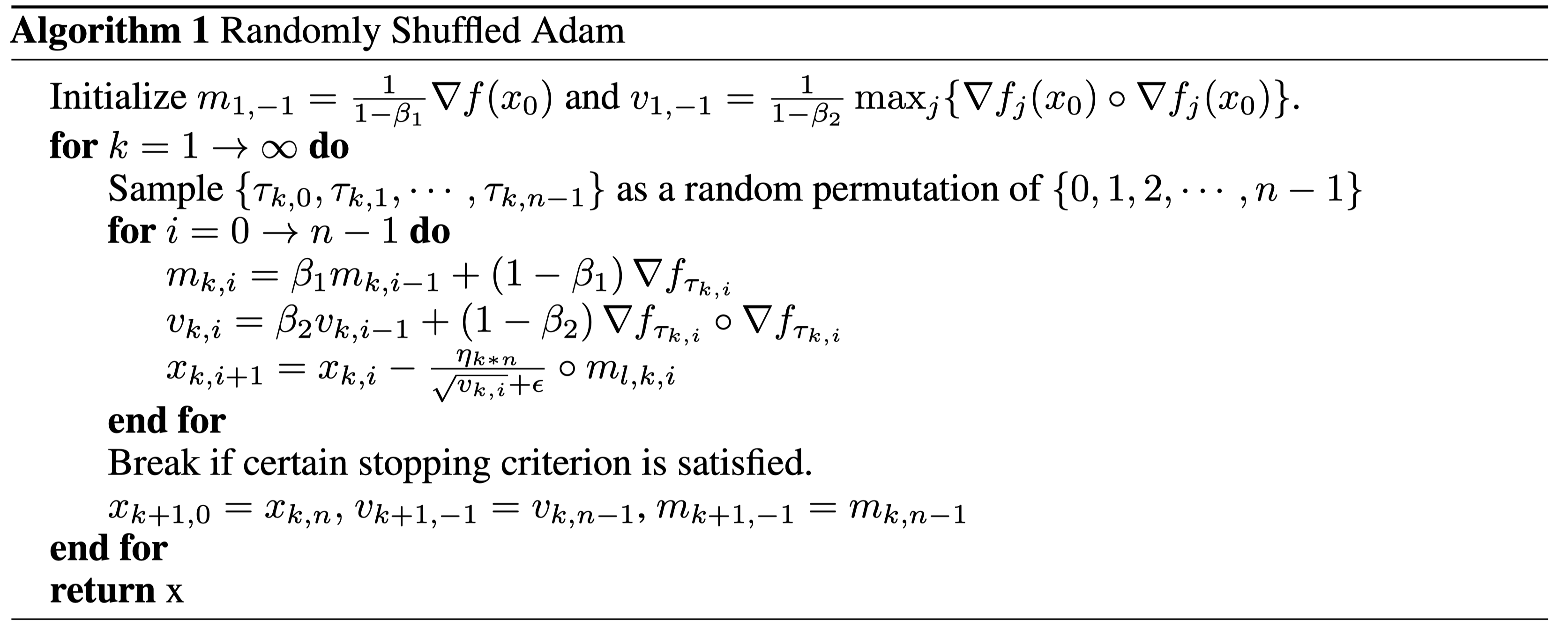
\[\begin{equation}\label{finite_sum} \min _{x \in \mathbb{R}^{d}} f(x)=\sum_{j=0}^{n-1} f_{j}(x). \end{equation} \tag{1}\]

In neural network training, $f_j(x)$ represents the loss function for the $j$-th sample batch; $x$ stands for the parameters in the neural networks. In Algorithm 1, we present the Randomly Shuffled Adam, which uses the strategy of sampling $f_j(x)$ without replacement. Compared with their with-replacement counterpart, randomly shuffling methods touch each data point at least once, and thus often have better performance [1,2]

In the vanilla version of Adam [8], it has an additional “bias correction’’ step. In Algorithm 1, this step is replaced by the initialization on $m_{1,-1}$ and $v_{1,-1}$, which also helps correct bias [17]. When $\beta_1=0,$ Algorithm 1 becomes RMSProp.

The results in [17] are based on the following assumptions.

Assumption 1. Assume $f_i$ are gradient Lipschitz continuous with constant $L$, and $f$ is lower bounded by a finite constant $f^*$.

Assumption 2. Assume \(\begin{equation} \sum_{i=0}^{n-1}\left\|\nabla f_{i}(x)\right\|_{2}^{2} \leq D_{1}\|\nabla f(x)\|_{2}^{2}+D_{0}. \end{equation}\)

When $D_1=n$, Assumption 2 becomes the “bounded variance’’ assumption with constant $D_0/n$. When $D_0=0$, Assumption 2 is often called “strong growth condition” (SGC) [20].

One sparkling contribution of [17] is that their analysis does not require the bounded gradient assumption, i.e., \(\begin{equation}\left\| \nabla f(x) \right\|< C, \forall x \end{equation}\). Removing this assumption is important for two reasons. First, the bounded gradient condition does not hold in the practical applications of Adam (deep neural nets training), not even for the simplest quadratic loss function $f(x)=x^2$. Second (and perhaps more importantly in this context), with bounded gradients assumptions, the gradients cannot diverge, while there is a counter-example showing that the gradient can diverge for certain problems [17].

We restate their convergence result as follows.

Theorem 1 (Theorem 4.3 in [17], informal) Consider the finite-sum problem (1) under Assumption 1 and 2. When $\beta_2 \geq 1- \mathcal{O}(n^{-3.5})$, RMSProp with stepsize $\eta_k = \eta_1/\sqrt{k}$ converges to a bounded region, namely:

\[\begin{equation} \min _{k \in(1, K]} \left\|\nabla f (x_{k,0})\right\|_{2}^{2} \leq \mathcal{O}\left(\frac{\log K}{\sqrt{K}}\right)+\mathcal{O}\left(\sqrt{D_{0}}\right). \end{equation}\]

It is expected that a stochastic algorithm only converges to a bounded region instead of a critical point, both in theory and practice. Indeed, the “convergence” of constant-stepsize SGD is in the sense of “converging to a region with size proportional to the noise variance”. Similar to SGD, in Theorem 1, the size of the region goes to zero as the noise variance goes to 0 or $D_0$ goes to 0.

Theorem 1 focuses on RMSProp, which is Adam with $\beta_1=0$. Motivated from Theorem 1, [17] also provides a convergence result for Adam with small enough $\beta_1$.

Theorem 2 (Theorem 4.4 in [17], informal) Consider the finite-sum problem (1) under Assumption 1 and 2. When $\beta_2 \geq 1- \mathcal{O}(n^{-3.5})$ and $\beta_1 \leq \mathcal{O}(n^{-2.5}) $, Adam with stepsize $\eta_k = \eta_1/\sqrt{k}$ converges to a bounded region, namely:

\[\begin{equation}\min _{k \in(1, K]} \left\|\nabla f (x_{k,0})\right\|_{2}^{2} \leq \mathcal{O}\left(\frac{\log K}{\sqrt{K}}\right)+\mathcal{O}\left(\sqrt{D_{0}}\right). \end{equation}\]

Reconcile the two papers. Reddi et al. [14] proved that Adam (including RMSProp) does not converge for a large set of hyperparameters, and [17] proved that RMSProp converges for large enough $\beta_2$. One might think that they are not contradictory because they cover different hyper-parameter settings; but this understanding is not correct and the actual relation is more subtle. Reddi et al. [14] showed that for any $\beta_2 \in [0 , 1) $ and $\beta_1 = 0 $, there exists a convex problem that RMSProp does not converge to optima. As a result, $ (\beta_1, \beta_2 ) = (0, 0.99) $ is a hyperparameter combination that can cause divergence; $ (\beta_1, \beta_2 ) = (0, 0.99999) $ can also cause divergence. In fact, no matter how much $\beta_2 $ is close to 1, $ (\beta_1, \beta_2 ) = (0, \beta_2 )$ can still cause divergence. So why does Shi et al. [17] claim “large enough $\beta_2$ makes RMSProp converge’’? The key lies in whether $ \beta_2$ is picked before or after picking the problem instance. What Shi et al. [17] proves is that: if $\beta_2$ is picked after the problem is given (thus $\beta_2$ can be problem-dependent), then RMSProp converges. This does not contradict the counter-example of [14] which picks $\beta_2$ before seeing the problem.

With the above discussion, we highlight two messages on the choice of $\beta_2$:

1. $\beta_2$ shall be large enough to ensure convergence;
2. The minimal-convergence-ensuring $\beta_2$ is a problem-dependent hyperparameter, rather than a universal hyperparameter.

$\beta_2$ is definitely not the first problem-dependent hyperparameter that we know. A much more well-known example is the stepsize: when the objective function is $L$-smooth, the stepsize of GD is a problem-dependent hyperparameter since it shall be less than $2/L$. For a given stepsize $\alpha $, one can always find a problem that GD with this stepsize diverges, but this does not mean “GD is non-convergent’’. The message above is: if we view $\beta_2 $ as a problem-dependent hyperparameter, then one can even say “RMSProp is convergent’’ in the sense that “RMSProp is convergent under proper choice of a problem-dependent hyperparameter’’.

[click here to go to the top][click here to go to the reference]

---

Gaps on the Convergence of Adam Left by Shi et al 2020

The above results by [17] take one remarkable step towards understanding Adam. Combining with the counter-example by [14], they show a phase transition from divergence to convergence when increasing $\beta_2$ from 0 to 1. However, Shi et al. [17] do not conclude the convergence discussion for Adam. In Theorem 1 and Theorem 2, they require $\beta_1$ to be either 0 or small enough. Is this a reasonable requirement? Does the requirement of $\beta_1$ match the practical use of Adam? If not, how large is the gap? We point out that this gap is actually non-negligible from multiple different perspectives. We elaborate as follows.

Gap with practice. We did some simple calculation regarding Theorem 2. To ensure convergence,
Theorem 2 requires $\beta_1 \leq \mathcal{O}(n^{-2.5})$. On CIFAR-10 with sample size 50,000 and batchsize 128, they need $\beta_1 < \mathcal{O}((50000/128)^{-2.5} ) \approx 10^{-7} $. This tiny value of $\beta_1$ is rarely used in practice. In fact, although there are certain scenarios where small $\beta_1$ is used (e.g. some methods for GAN and RL such as [16] and [12]), but in these cases, often 0 or 0.1 are used, rather than a tiny non-zero value $10^{-7}$. For most applications of Adam, larger $\beta_1$ is used. Kingma and Ba [8] claimed that $\beta_1=0.9$ is a “good default setting for the tested machine learning problems.” Later on, $\beta_1=0.9$ is also adopted in PyTorch default setting.

Lack in providing useful message on $\beta_1$. One might argue that Theorem 2 just provided a theoretical bound on $\beta_1$ and does not have to match practical values. In fact, the required bound on $\beta_2$ of Theorem 1 is $1 - \mathcal{O}(n^{-3.5})$. This value is also larger than the practical value of $\beta_2 $ such as $0.999 = 1-0.001$. However, there is a major difference between the lower bound of $\beta_2$ and the upper bound of $\beta_1$: the former provides a conceptual message that $\beta_2$ shall be large enough to ensure good performance which matches experiments, while the latter does not seem to provide any useful message.

Theoretical gap in the context of [14]. The counter-example of [14] applies to any $(\beta_1, \beta_2)$ such that $ \beta_1 < \sqrt{\beta_2 }$. The counter-example is valid and there is no way to prove Adam converges for general problems for this hyperparameter combination. Nevertheless, as argued earlier, the caveat is on problem independent hyperparameters. As argued earlier, Shi et al. [17] noticed the counter-example of [14] applies to problem-independent hyperparameters, and switching the order of problem-picking and hyper-parameter-picking can lead to convergence. But this switching-order-argument only applies to $\beta_2$ and not necessarily applies to $\beta_1$. When $\beta_2$ is problem-dependent, it is not clear whether Adam converges for larger $\beta_1$.

Next, we discuss the importance of understanding Adam with large $\beta_1$.

Possible empirical benefit for understanding Adam with large $\beta_1$. (We call $\beta_1$ “large” when it is, at least, larger than 0.1.) In the above, we have discussed the theoretical, empirical , and conceptual gap on the understanding of Adam’s convergence. We next discuss one possible empirical benefit for filling in this gap: guiding practitioners to better tune hyperparameters. At the current stage, many practitioners are trapped in the default setting with no idea how to better tune $\beta_1$ and $\beta_2$. Shi et al. [17] provide a simple guidance on tuning $\beta_2$ when $\beta_1 = 0$: start from $\beta_2 = 0.8 $ and tune $\beta_2$ up until reaching the best performance. Nevertheless, there is not much guidance on tuning $\beta_1$. If Adam does not solve your tasks well in the default setting $\beta_1=0.9$, how should you tune the hyperparameter to make it work? Shall you tune it up or down or both? When you tune $\beta_1$, shall you tune $\beta_2$ as well? A more confusing phenomenon is that both large $\beta_1$ like $\beta_1 = 0.9$ and small $\beta_1 $ like $\beta_1 = 0$ are used in different papers. This makes it hard to guess what is a proper way of tuning $\beta_1$ (together with tuning $\beta_2$).

How difficult could it be to adopt large $\beta_1$ into convergence analysis? We are inclined to believe it is not easy. Momentum contains a heavy amount of history information which dramatically distorts the trajectory of the iterates. Technically speaking, Shi et al. [17] treat momentum as a pure error deviating from the gradient direction. Following this proof idea, this error can only be controlled when $\beta_1$ is closed enough to 0. To cover large $\beta_1$ into convergence analysis, one needs to handle momentum from a different perspective.

[click here to go to the top][click here to go to the reference]

---

Conclusions

In this blog post, we briefly review the non-convergence results by [14] and the convergence results by [17]. Their results take remarkable steps forward to understand Adam better. Meanwhile, they also expose many new questions that are not yet discussed. Compared with its practical success, the current theoretical understanding for Adam is still left behind.

[click here to go to the top]

---

Disclosure of Funding

The work of Z.-Q. Luo is supported by the National Natural Science Foundation of China (No. 61731018) and the Guangdong Provincial Key Laboratory of Big Data Computation Theories and Methods.

---

References

• [1] L. Bottou. Curiously fast convergence of some stochastic gradient descent algorithms. InProceedings of the symposium on learning and data science, Paris, volume 8, pages 2624–2633,2009.
• [2] L. Bottou. Stochastic gradient descent tricks. InNeural networks: Tricks of the trade, pages421–436. Springer, 2012. </li>
• [3] T. B. Brown, B. Mann, N. Ryder, M. Subbiah, J. Kaplan, P. Dhariwal, A. Neelakantan,P. Shyam, G. Sastry, A. Askell, et al. Language models are few-shot learners.arXiv preprintarXiv:2005.14165, 2020.
• [4] J. Devlin, M.-W. Chang, K. Lee, and K. Toutanova. Bert: Pre-training of deep bidirectionaltransformers for language understanding.arXiv preprint arXiv:1810.04805, 2018.
• [5] T. Dozat. Incorporating nesterov momentum into adam. 2016.
• [6] J. Duchi, E. Hazan, and Y. Singer. Adaptive subgradient methods for online learning andstochastic optimization.Journal of machine learning research, 12(7), 2011.
• [7] P. Isola, J.-Y. Zhu, T. Zhou, and A. A. Efros. Image-to-image translation with conditionaladversarial networks. InProceedings of the IEEE conference on computer vision and patternrecognition, pages 1125–1134, 2017.
• [8] D. P. Kingma and J. Ba. Adam: A method for stochastic optimization.arXiv preprintarXiv:1412.6980, 2014.
• [9] T. P. Lillicrap, J. J. Hunt, A. Pritzel, N. Heess, T. Erez, Y. Tassa, D. Silver, and D. Wierstra.Continuous control with deep reinforcement learning.arXiv preprint arXiv:1509.02971, 2015.
• [10] L. Luo, Y. Xiong, Y. Liu, and X. Sun. Adaptive gradient methods with dynamic bound oflearning rate.arXiv preprint arXiv:1902.09843, 2019.- [11]H. B. McMahan and M. Streeter. Adaptive bound optimization for online convex optimization.arXiv preprint arXiv:1002.4908, 2010.
• [12] V. Mnih, A. P. Badia, M. Mirza, A. Graves, T. Lillicrap, T. Harley, D. Silver, and K. Kavukcuoglu.Asynchronous methods for deep reinforcement learning. InInternational conference on machinelearning, pages 1928–1937. PMLR, 2016.
• [13] A. Radford, L. Metz, and S. Chintala. Unsupervised representation learning with deep convolu-tional generative adversarial networks.arXiv preprint arXiv:1511.06434, 2015.
• [14] S. J. Reddi, S. Kale, and S. Kumar. On the convergence of adam and beyond.arXiv preprintarXiv:1904.09237, 2019.
• [15] J. Schulman, F. Wolski, P. Dhariwal, A. Radford, and O. Klimov. Proximal policy optimizationalgorithms.arXiv preprint arXiv:1707.06347, 2017.
• [16] C. Seward, T. Unterthiner, U. Bergmann, N. Jetchev, and S. Hochreiter. First order generativeadversarial networks. InInternational Conference on Machine Learning, pages 4567–4576.PMLR, 2018.
• [17] N. Shi, D. Li, M. Hong, and R. Sun. Rmsprop converges with proper hyper-parameter. InInternational Conference on Learning Representations, 2020.
• [18] T. Tieleman and G. Hinton. Divide the gradient by a running average of its recent magnitude.coursera: Neural networks for machine learning.Technical Report, 2017.
• [19] A. Vaswani, N. Shazeer, N. Parmar, J. Uszkoreit, L. Jones, A. N. Gomez, Ł. Kaiser, andI. Polosukhin. Attention is all you need. InAdvances in neural information processing systems,pages 5998–6008, 2017.
• [20] S. Vaswani, F. Bach, and M. Schmidt. Fast and faster convergence of sgd for over-parameterizedmodels and an accelerated perceptron. InThe 22nd International Conference on ArtificialIntelligence and Statistics, pages 1195–1204. PMLR, 2019.
• [21] M. D. Zeiler. Adadelta: an adaptive learning rate method.arXiv preprint arXiv:1212.5701,2012.
• [22] J.-Y. Zhu, T. Park, P. Isola, and A. A. Efros. Unpaired image-to-image translation usingcycle-consistent adversarial networks. InProceedings of the IEEE international conference oncomputer vision, pages 2223–2232, 2017.

[click here to go to the top]