Learning to Coarsen Graphs with Graph Neural Networks

With the rise of large-scale graphs for relational learning, graph coarsening emerges as a computationally viable alternative. We revisit the principles that aim to improve data-driven graph coarsening with adjustable coarsened structures.

Graph Coarsening 101

TLDR- Coarsening methods group nearby nodes to a supernode while preserving their relational properties. Traditional approaches only aim at node assignment with limited weight adjustment and similarity assessment.

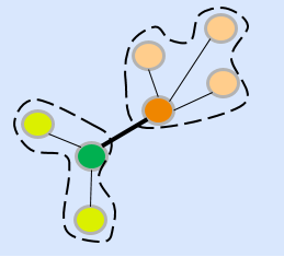
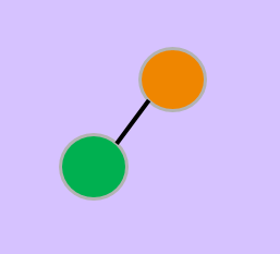
Graph coarsening relates to the process of preserving node properties of a graph by grouping them into similarity clusters. These similarity clusters form the new nodes of the coarsened graph and are hence termed as supernodes. Contrary to partitioning methods graph partitioning is the process of segregating a graph into its sub-graphs. which aim to extract information of local neighborhoods, coarsening aims to extract global representations of a graph. This implies that the coarsened graph must have all the node properties of the original graph preserved up to a certain level of accuracy.

Modern coarsening approaches aim to retain the spectral properties between original and coarse graphs. This involves the usage of spectral approximations and probabilistic frameworks to link nodes between the two structures. Although helpful, learning node assignments often results in lost edge information within nodes. Edge weights, during coarsening, are held fixed proportional to the total weights of incident edges between two given nodes. This hinders one to learn the connectivity of coarsened graphs.

In addition to connectivity, a spectral analysis of the coarsened graph is difficult to obtain. Assessing properties of different graph structures requires information about each node. Coarse graph supernodes, however, are themselves compositions of high-granularity nodes. This prevents a direct comparison between original and coarse representations. Let's formalize this problem in detail.

$$G = (V,E)$$

$$\pi : V \rightarrow \hat{V}$$

$$L = D - W$$

assign nodes: $\checkmark$

compare structure: $\times$

adjust weights: $\times$

$$\hat{G} = (\hat{V},\hat{E})$$

$$\pi^{-1} : \hat{V} \rightarrow V$$

$$\hat{L} = \hat{D} - \hat{W}$$

The graph coarsening process (flip cards for details).

An original graph $G = (V,E)$ has $N = |V|$ nodes and standard Laplace operator Laplacians summarize spectral properties of graphs with symmetric and positive semi-definite structure. $L = D-W$ expressing the difference between the degree matrix $D$ and edge weight matrix $W$. The coarsened graph $\hat{G} = (\hat{V},\hat{E})$ has $n = |\hat{V}|$ nodes ($n < N$) and the Laplacian $\hat{L} = \hat{D}-\hat{W}$. $G$ and $\hat{G}$ are linked via the vertex map $\pi: V \rightarrow \hat{V}$ such that all nodes $\pi^{-1}(\hat{v}) \in V$ are mapped to the supernode $\hat{v}$. The vertex map is thus a surjective mapping from the original graph to coarse graph. Due to a diference in the number of nodes, the two graphs denote different structures and hence, the Laplacians $L$ and $\hat{L}$ are not directy comparable.

Operations to Coarsen Graphs

TLDR- Assessment of Laplacian leads to a lift & project mapping formulation. In what follows, the formulation constructs a similarity measure $\mathcal{L}$ based on edge and vertex weights.

Establishing a link between original and coarsened graph requires a brief visit into their operators. To compare two graphs the paper defines operators on both original and coarse graphs. Let's begin by revisiting these operators for both structures.

Laplace This Way

Since $G$ and $\hat{G}$ have different number of nodes, their Laplace operators $L$ and $\hat{L}$ are not directly comparable. Instead, we can utilize a functional mapping $\mathcal{F}$ which would remain invariant to the vertices of $G$ and $\hat{G}$. Such a mapping is intrinsic to the graph of interest, i.e.- the mapping would operate on $N$ vectors $f$ as well as $n$ vectors $\hat{f}$. This allows us to compare between $\mathcal{F}(L,f)$ and $\mathcal{F}(\hat{L},\hat{f})$.

For the vertex map $\pi$, we set an $n \times N$ matrix P as,

for any $r \in [1,n]$. It is worth noting that the map $\pi$ may not always be given to us and can be approximated using a learning process. Next, we denote $P^{+}$ as the $N \times n$ pseudo-inverse Formally known as the Moore-Penrose inverse, the pseudo-inverse is an approximate inverse to matrices which may not invertible. of P. Note that $P^{+}$ operates on the set $\hat{V}$ to provide a mapping in $V$. This allows us to formulate an operator on the coarsened set $\hat{V}$,

$$\begin{equation} \tilde{L} = (P^{+})^{T}LP^{+} \end{equation}$$

$\tilde{L}$ operates on $n$ vectors $\hat{f} \in \mathbb{R}^{n}$ corresponding to the coarsened set. We look deeper into this mapping next.

Lift & Project

We can intuitively understand the mapping $\tilde{L}$ as a lift and project mapping. Let's break this computation step-by-step. For a $n$ vector $\hat{f}$, the first operation $f = P^{+}\hat{f}$ lifts the $n$ dimensional representation to an $N$ dimensional one. The operation of $L$ then yields the desired result for spectral comparison. Following this computation, $Lf$ is again projected down to the $n$ vector space by the operation of $(P^{+})^{T}$.

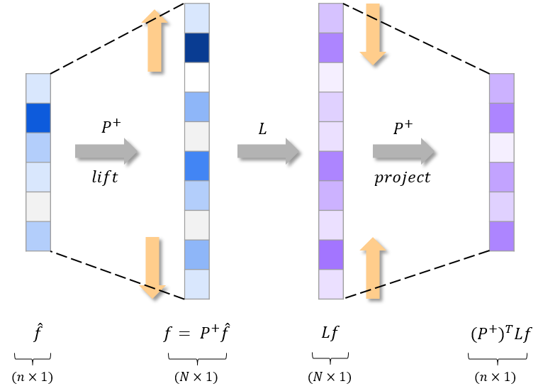
Lift and Project mappings between $n$ and $N$ vectors.

Simultaneous actions of lift and project mappings give rise to a general framework between original and coarsened objects of the graph. The $\tilde{L}$ formulation for the above construction resembles the quadratic form $Q_{A}(x) = x^{T}Ax$ with $x^{T}$ as the lift $P^{+}$, $A$ as the Laplacian $L$ and $x$ as the projection map $P$. Similarly, an alternate construction could be obtained by considering the Rayleigh Quotient form,

Why the Rayleigh formulation? This is because the eigenvectors and eigenvalues of the linear operator $A$ are more directly related to its Rayleigh Quotient. The Rayleigh Quotient informs us about the geometry of its vectors in high-dimensional spaces. Thus, we change our formulation and construct a doubly-weighted Laplace operator. This operator has the special property that it retains both edge and vertex information by explicitly weighing them during operation. For the coarse graph $\hat{G}$ with each vertex $\hat{v} \in \hat{V}$ weighted by $\gamma = |\pi^{-1}(\hat{v})|$, let $\Gamma$ be the diagonal $n \times n$ vertex matrix with entries $\Gamma[r][r] = \gamma_{r}$, the doubly-weighted Laplace operator is then defined as,

$\mathcal{L} = $ $\Gamma^{-\frac{1}{2}}$$\hat{L}$$\Gamma^{-\frac{1}{2}}$$ = $$\underbrace{(P^{+}\Gamma^{-\frac{1}{2}})^{T}}_{\text{lift}}$$L$$\underbrace{(P^{+}\Gamma^{-\frac{1}{2}})}_{\text{project}}$

This motivates us to use $\mathcal{L}$ as a similarity measure during the coarsening process.

Learning Graph Coarsening

TLDR- GOREN utilizes a GNN to assign edge weights by minimizing an unsupervised loss between functional mappings $\mathcal{F}(L,f)$ and $\mathcal{F}(\hat{L},\hat{f})$. Weight adjustment yields improved quadratic and eigen error reduction.

We now utilize the Rayleigh Quotient formulation to construct a framework for learning coarsening of graphs. The core of learning process is formed by the motivation to reset and learn edge weight assignments of the coarse graph.

The GOREN Framework

Following previous section, we know that the usage of better Laplace operators leads to better-informed strictly in the spectral sense. weights. Using this insight, the setting develops a framework wherein the weight $\hat{w}(\hat{v},\hat{v}^{\prime})$ on the edge $(\hat{v},\hat{v}^{\prime})$ is predicted using a weight-assignment function $\mu(G_{A})$. Here, $G_{A}$ denotes the subgraph induced by a subset of vertices $A$. Note that there are two problems with $\mu(G_{A})$; (1) it is unclear as to what the stucture of this function should be and (2) the functional arguments can scale rapidly for large number of nodes in $A$. This is where Graph Neural Networks (GNNs) come in.

GNNs are employed as effective parameterizations to learn a collection of input graphs in unsupervised fashion. The weight-assignment map $\mu$ corresponds to a learnable neural network. This Graph cOarsening RefinemEnt Network (GOREN) reasons about local regions as supernodes and assigns a weight to each edge in the coarse graph. GOREN uses the Graph Isomorphism Network (GIN) as its GNN model. All edge attributes of the coarse graph are initialized to 1. Weights assigned by the network are enforced to be positive using an additional ReLU output layer.

GOREN enables weight adjustment using similarity measures between $G$ and $\hat{G}$.

GOREN is trained to minimize the distance between functional mappings $\mathcal{F}(L,f)$ and $\mathcal{F}(\hat{L},\hat{f})$ with $\hat{f}$ as the projection of $f$ and $k$ as the number of node atttributes,

$ \text{Loss}(L,\hat{L}) = \frac{1}{k}\sum_{i=1}^{k}|$$\underbrace{\mathcal{F}(L,f_{i})}_{\text{original graph}}$$ - $$\underbrace{\mathcal{F}(\hat{L},\hat{f}_{i})}_{\text{coarsened graph}}$$|$

def goren(graph, net):
    weights = net.forward(graph)
    coarse_graph = construct_graph(weights)
    l = compute_l(graph)
    l_hat = compute_l_hat(coarse_graph)
    loss = 0.5*(l - l_hat)**2
    loss = loss.mean().backward()
    return loss.data

Practical implementation of the algorithm uses Rayleigh formulation with $\mathcal{F}$ as the Rayleigh Quotient, $\hat{L}$ as the double-weighted Laplacian $\mathcal{L}$, and $\hat{f}$ as the lift-project mapping $\hat{f} = (P^{+})^{T}L$. At test time, a graph $G_{\text{test}}$ is passed through the network to predict edge weights for the new graph $\hat{G}_{\text{test}}$ by minimizing the loss iteratively.

Weight Assignments & Adjustments

Primary component which rests behind the success of GOREN is its weight assignment and adjustment scheme. Using a GNN allows GOREN to reset and adjust edge weights. These weights capture local structure from neighborhoods of the original graph. This small trick can be applied on top of previous coarsening algorithms and improve node connectivity.

GOREN outperforms MLP weight assignment in error reduction on (left) WS and (right) shape datasets.

When compared to MLP-based weight assignment on various coarsening algorithms; namely random BaseLine (BL), Affinity, Algebraic Distance, Heavy edge matching, Local variation (in edges) and Local variation (in neighbors); GOREN demonstrates greater % improvement in error reduction. Especially on the shape dataset where MLPs fail to assign weights, GOREN presents significant minimization in error. This results in better connectivity of the coarsened graph with spectral properties preserved of the original graph.

Closing Remarks

TLDR- Learning the coarsening process can be further improved by extending GOREN towards (1) learnable node assignment, (2) non-differentiable loss functions and (3) similarity with downstream tasks.

We looked at graph coarsening in the presence of edge weights. A weight assignment and adjustment scheme is constructed using the GOREN framework. GNNs are trained in an unsupervised fashion to preserve the spectral properties of original graph. While our discussion has been restricted to the study of GOREN, we briefly extend the scope towards other future avenues.

Beyond Graph Coarsening

An important aspect to consider is the node topology of graphs. While GOREN operates on node-coarsened structures, it would be interesting to extend the framework towards a full coarsening approach. Grouping in supernodes can be learned using a separate GNN following GOREN. Such algorithms would lead to the generation of end-to-end graph coarsening methods. This will reduce our dependence on handcrafted coarsening techniques.

Another line of work originates from different types of losses. GOREN utilizes differentiable loss functions including mappings. The study can be further extended to non-differentiable loss functions which require challenging computations, e.g- inverse Laplacian. These functions consist of mappings with hidden spectral features which are difficult to obtain.

Lastly, GOREN could explicitly reason about which properties are important to preserve. This would provide interesting insights into various metrics and their utility in downstream learning of coarsened graphs.

Further Reading

1. Chen Cai, Dingkang Wang, Yusu Wang, Graph Coarsening with Neural Networks, ICLR 2021.

2. Andreas Loukas, Pierre Vandergheynst, Spectrally approximating large graphs with smaller graphs, ICLR 2018.

3. Gecia Bravo-Hermsdorf, Lee M. Gunderson, A Unifying Framework for Spectrum-Preserving Graph Sparsification and Coarsening, NeurIPS 2019.

4. Benjamin Sanchez-Lengeling, Emily Reif, Adam Pearce, Alexander B. Wiltschko, A Gentle Introduction to Graph Neural Networks, Distill 2021.

5. Ameya Daigavane, Balaraman Ravindran, Gaurav Aggarwal, Understanding Convolutions on Graphs, Distill 2021.

6. Danijela Horak, Jürgen Jost, Spectra of combinatorial Laplace operators on simplicial complexes, AIM 2013.

7. Andreas Loukas, Graph reduction with spectral and cut guarantees, JMLR 2019.

8. Hermina Petric Maretic, Mireille EL Gheche, Giovanni Chierchia, Pascal Frossard, GOT: An Optimal Transport framework for Graph comparison, NeurIPS 2019.