The Annotated S4

Blog Post and Library by Sasha Rush and Sidd Karamcheti, v2

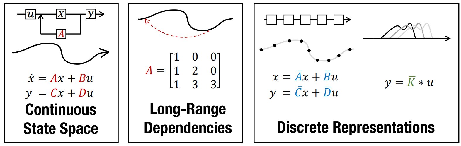
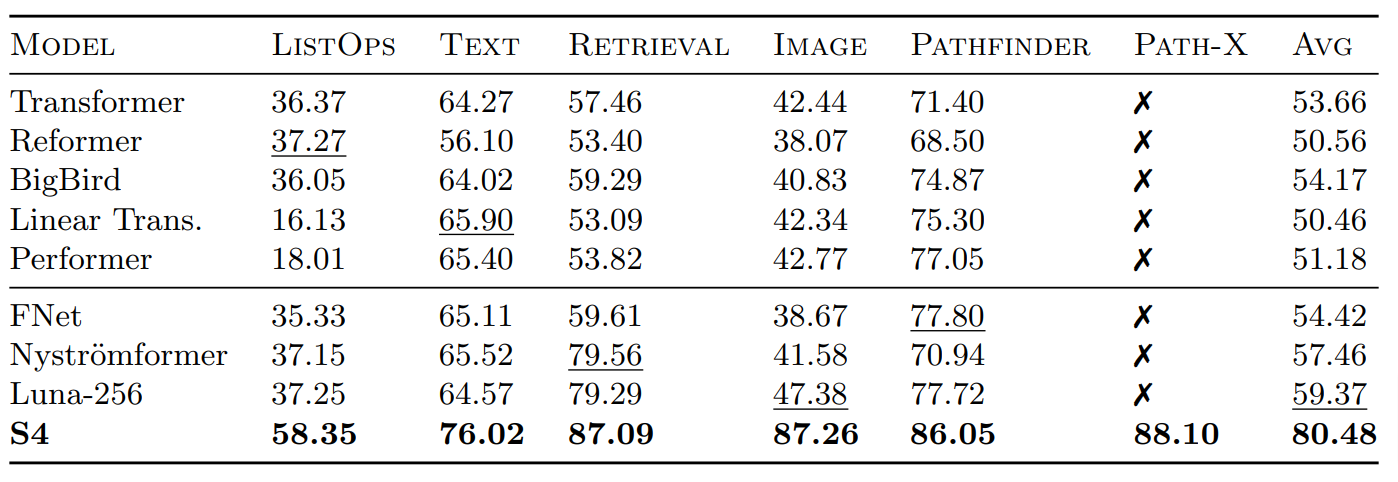
The Structured State Space for Sequence Modeling (S4) architecture is a new approach to very long-range sequence modeling tasks for vision, language, and audio, showing a capacity to capture dependencies over tens of thousands of steps. Especially impressive are the model’s results on the challenging Long Range Arena benchmark, showing an ability to reason over sequences of up to 16,000+ elements with high accuracy.

The paper is also a refreshing departure from Transformers, taking a very different approach to an important problem-space. However, several of our colleagues have also noted privately the difficulty of gaining intuition for the model. This blog post is a first step towards this goal of gaining intuition, linking concrete code implementations with explanations from the S4 paper – very much in the style of the annotated transformer. Hopefully this combination of code and literate explanations helps you follow the details of the model. By the end of the blog you will have an efficient working version of S4 that can operate as a CNN for training, but then convert to an efficient RNN at test time. To preview the results, you will be able to generate images from pixels and sounds directly on sound waves on a standard GPU.

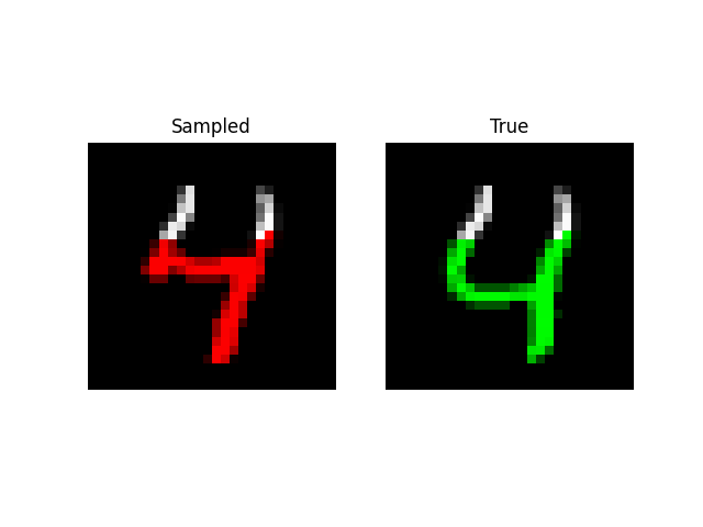
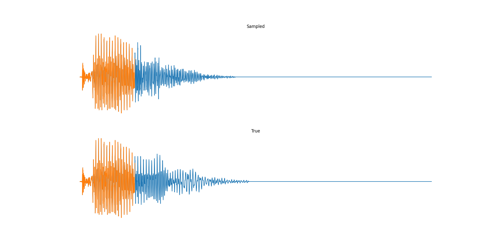
Table of Contents

Note that this project uses JAX with the Flax NN library. While we personally mainly use Torch, the functional nature of JAX is a good fit for some of the complexities of S4. We make heavy use of vmap, scan, their NN cousins, and most importantly jax.jit to compile fast and efficient S4 layers.

from functools import partial
import jax
import jax.numpy as np
from flax import linen as nn
from jax.nn.initializers import lecun_normal, uniform
from jax.numpy.linalg import eig, inv, matrix_power
from jax.scipy.signal import convolve

rng = jax.random.PRNGKey(1)

Part 1: State Space Models

Let’s get started! Our goal is the efficient modeling of long sequences. To do this, we are going to build a new neural network layer based on State Space Models. By the end of this section we will be able to build and run a model with this layer. However, we are going to need some technical background. Let’s work our way through the background of the paper.

The state space model is defined by this simple equation. It maps a 1-D input signal $u(t)$ to an $N$-D latent state $x(t)$ before projecting to a 1-D output signal $y(t)$.

Our goal is to simply use the SSM as a black-box representation in a deep sequence model, where $\boldsymbol{A}, \boldsymbol{B}, \boldsymbol{C}, \boldsymbol{D}$ are parameters learned by gradient descent. For the remainder, we will omit the parameter $\boldsymbol{D}$ for exposition (or equivalently, assume $\boldsymbol{D} = 0$ because the term $\boldsymbol{D}u$ can be viewed as a skip connection and is easy to compute).

An SSM maps a input $u(t)$ to a state representation vector $x(t)$ and an output $y(t)$. For simplicity, we assume the input and output are one-dimensional, and the state representation is $N$-dimensional. The first equation defines the change in $x(t)$ over time.

Our SSMs will be defined by three matrices – $\boldsymbol{A}, \boldsymbol{B}, \boldsymbol{C}$ – which we will learn. For now we begin with a random SSM, to define sizes,

def random_SSM(rng, N):
    a_r, b_r, c_r = jax.random.split(rng, 3)
    A = jax.random.uniform(a_r, (N, N))
    B = jax.random.uniform(b_r, (N, 1))
    C = jax.random.uniform(c_r, (1, N))
    return A, B, C

Discrete-time SSM: The Recurrent Representation

To be applied on a discrete input sequence $(u_0, u_1, \dots )$ instead of continuous function $u(t)$, the SSM must be discretized by a step size $\Delta$ that represents the resolution of the input. Conceptually, the inputs $u_k$ can be viewed as sampling an implicit underlying continuous signal $u(t)$, where $u_k = u(k \Delta)$.

To discretize the continuous-time SSM, we use the bilinear method, which converts the state matrix $\boldsymbol{A}$ into an approximation $\boldsymbol{\overline{A}}$. The discrete SSM is:

def discretize(A, B, C, step):
    I = np.eye(A.shape[0])
    BL = inv(I - (step / 2.0) * A)
    Ab = BL @ (I + (step / 2.0) * A)
    Bb = (BL * step) @ B
    return Ab, Bb, C

This equation is now a sequence-to-sequence map $u_k \mapsto y_k$ instead of function-to-function. Moreover the state equation is now a recurrence in $x_k$, allowing the discrete SSM to be computed like an RNN. Concretely, $x_k \in \mathbb{R}^N$ can be viewed as a hidden state with transition matrix $\boldsymbol{\overline{A}}$.

As the paper says, this “step” function does look superficially like that of an RNN. We can implement this with a scan in JAX,

def scan_SSM(Ab, Bb, Cb, u, x0):
    def step(x_k_1, u_k):
        x_k = Ab @ x_k_1 + Bb @ u_k
        y_k = Cb @ x_k
        return x_k, y_k

    return jax.lax.scan(step, x0, u)

Putting everything together, we can run the SSM by first discretizing, then iterating step by step,

def run_SSM(A, B, C, u):
    L = u.shape[0]
    N = A.shape[0]
    Ab, Bb, Cb = discretize(A, B, C, step=1.0 / L)

    # Run recurrence
    return scan_SSM(Ab, Bb, Cb, u[:, np.newaxis], np.zeros((N,)))[1]

Tangent: A Mechanics Example

To gain some more intuition and test our SSM implementation, we pause from machine learning to implement a classic example from mechanics.

In this example, we consider the forward position $y(t)$ of a mass attached to a wall with a spring. Over time, varying force $u(t)$ is applied to this mass. The system is parameterized by mass ($m$), spring constant ($k$), friction constant ($b$). We can relate these with the following differential equation:

Rewriting this in matrix form yields an SSM in the following form:

def example_mass(k, b, m):
    A = np.array([[0, 1], [-k / m, -b / m]])
    B = np.array([[0], [1.0 / m]])
    C = np.array([[1.0, 0]])
    return A, B, C

Looking at the $\boldsymbol{C}$, we should be able to convince ourselves that the first dimension of the hidden state is the position (since that becomes $y(t)$). The second dimension is the velocity, as it is impacted by $u(t)$ through $\boldsymbol{B}$. The transition $\boldsymbol{A}$ relates these terms.

We’ll set $u$ to be a continuous function of $t$,

@partial(np.vectorize, signature="()->()")
def example_force(t):
    x = np.sin(10 * t)
    return x * (x > 0.5)

Let’s run this SSM through our code.

def example_ssm():
    # SSM
    ssm = example_mass(k=40, b=5, m=1)

    # L samples of u(t).
    L = 100
    step = 1.0 / L
    ks = np.arange(L)
    u = example_force(ks * step)

    # Approximation of y(t).
    y = run_SSM(*ssm, u)

    # Plotting ---
    import matplotlib.pyplot as plt
    import seaborn
    from celluloid import Camera

    seaborn.set_context("paper")
    fig, (ax1, ax2, ax3) = plt.subplots(3)
    camera = Camera(fig)
    ax1.set_title("Force $u_k$")
    ax2.set_title("Position $y_k$")
    ax3.set_title("Object")
    ax1.set_xticks([], [])
    ax2.set_xticks([], [])

    # Animate plot over time
    for k in range(0, L, 2):
        ax1.plot(ks[:k], u[:k], color="red")
        ax2.plot(ks[:k], y[:k], color="blue")
        ax3.boxplot(
            [[y[k, 0] - 0.04, y[k, 0], y[k, 0] + 0.04]],
            showcaps=False,
            whis=False,
            vert=False,
            widths=10,
        )
        camera.snap()
    anim = camera.animate()
    anim.save("line.gif", dpi=150, writer="imagemagick")

if False:
    example_ssm()

Neat! And that it was just 1 SSM, with 2 hidden states over 100 steps. The final model will have had 100s of stacked SSMs over thousands of steps. But first – we need to make these models practical to train.

Training SSMs: The Convolutional Representation

The punchline of this section is that we can turn the “RNN” above into a “CNN” by unrolling. Let’s go through the derivation.

The recurrent SSM is not practical for training on modern hardware due to its sequential nature. Instead, there is a well-known connection between linear time-invariant (LTI) SSMs and continuous convolutions. Correspondingly, the recurrent SSM can actually be written as a discrete convolution.

For simplicity let the initial state be $x_{-1} = 0$. Then unrolling explicitly yields:

This can be vectorized into a convolution with an explicit formula for the convolution kernel.

We call $\boldsymbol{\overline{K}}$ the SSM convolution kernel or filter.

Note that this is a giant filter. It is the size of the entire sequence!

def K_conv(Ab, Bb, Cb, L):
    return np.array(
        [(Cb @ matrix_power(Ab, l) @ Bb).reshape() for l in range(L)]
    )

Warning: this implementation is naive and unstable. In practice it will fail to work for more than very small lengths. However, we are going to replace it with S4 in Part 2, so for now we just keep it around as a placeholder.

We can compute the result of applying this filter either with a standard direct convolution or by using convolution theorem with Fast Fourier Transform (FFT). The discrete convolution theorem - for circular convolution of two sequences - allows us to efficiently calculate the output of convolution by first multiplying FFTs of the input sequences and then applying an inverse FFT. To utilize this theorem for non-circular convolutions as in our case, we need to pad the input sequences with zeros, and then unpad the output sequence. As the length gets longer this FFT method will be more efficient than the direct convolution,

def non_circular_convolution(u, K, nofft=False):
    if nofft:
        return convolve(u, K, mode="full")[: u.shape[0]]
    else:
        assert K.shape[0] == u.shape[0]
        ud = np.fft.rfft(np.pad(u, (0, K.shape[0])))
        Kd = np.fft.rfft(np.pad(K, (0, u.shape[0])))
        out = ud * Kd
        return np.fft.irfft(out)[: u.shape[0]]

The CNN method and the RNN method yield (roughly) the same result,

def test_cnn_is_rnn(N=4, L=16, step=1.0 / 16):
    ssm = random_SSM(rng, N)
    u = jax.random.uniform(rng, (L,))
    jax.random.split(rng, 3)
    # RNN
    rec = run_SSM(*ssm, u)

    # CNN
    ssmb = discretize(*ssm, step=step)
    conv = non_circular_convolution(u, K_conv(*ssmb, L))

    # Check
    assert np.allclose(rec.ravel(), conv.ravel())

At this point we have all of the machinery used for SSM training. The next steps are about 1) making these models stable to train, and 2) making them fast.

Addressing Long-Range Dependencies with HiPPO

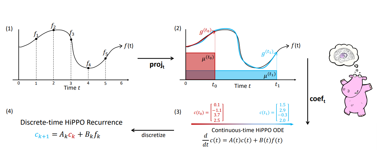
Prior work found that the basic SSM actually performs very poorly in practice. Intuitively, one explanation is that they suffer from gradients scaling exponentially in the sequence length (i.e., the vanishing/exploding gradients problem). To address this problem, previous work developed the HiPPO theory of continuous-time memorization.

HiPPO specifies a class of certain matrices $\boldsymbol{A} \in \mathbb{R}^{N \times N}$ that when incorporated, allow the state $x(t)$ to memorize the history of the input $u(t)$. The most important matrix in this class is defined by the HiPPO matrix.

Previous work found that simply modifying an SSM from a random matrix $\boldsymbol{A}$ to HiPPO improved its performance on the sequential MNIST classification benchmark from $50\%$ to $98\%$.

This matrix is going to be really important, but it is a bit of magic. For our purposes we mainly need to know that: 1) we only need to calculate it once, and 2) it has a nice, simple structure (which we will exploit in part 2). Without going into the ODE math, the main takeaway is that this matrix aims to remember the past history in the state a timescale invariant manner,

def make_HiPPO(N):
    def v(n, k):
        if n > k:
            return np.sqrt(2 * n + 1) * np.sqrt(2 * k + 1)
        elif n == k:
            return n + 1
        else:
            return 0

    # Do it slow so we don't mess it up :)
    mat = [[v(n, k) for k in range(1, N + 1)] for n in range(1, N + 1)]
    return np.array(mat)

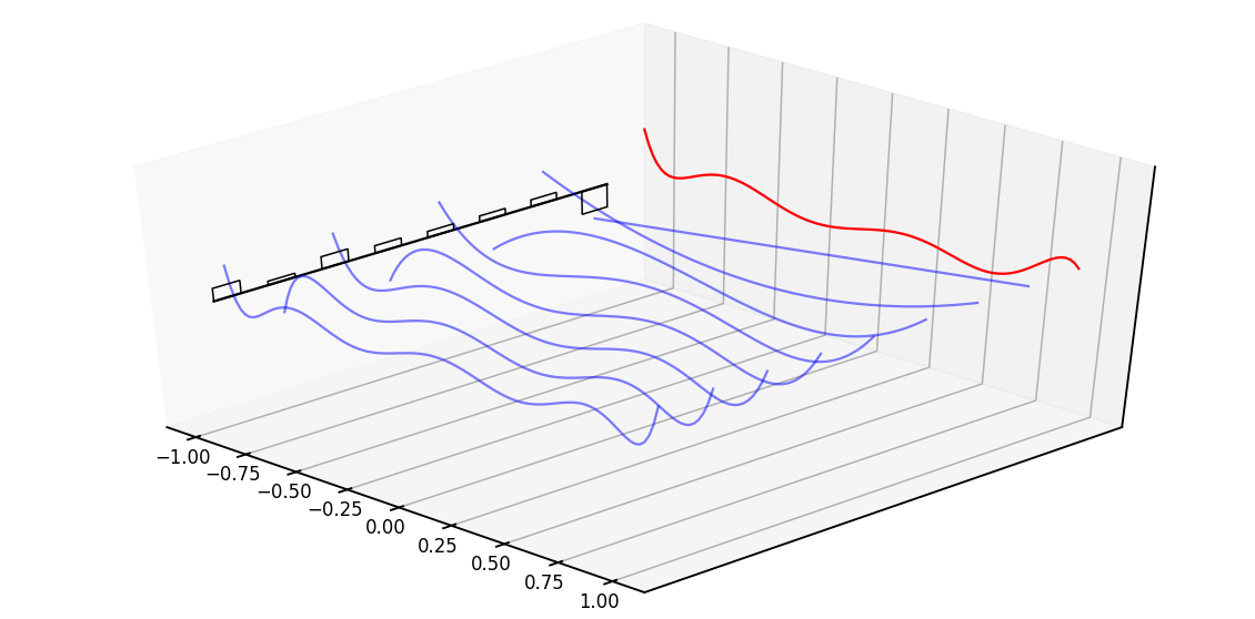
Diving a bit deeper, the intuitive explanation of this matrix is that it produces a hidden state that memorizes its history. It does this by keeping track of the coefficients of a Legendre polynomial. These coefficients let it approximate all of the previous history. Let us look at an example,

def example_legendre(N=8):
    # Random hidden state as coefficients
    import numpy as np
    import numpy.polynomial.legendre

    x = (np.random.rand(N) - 0.5) * 2
    t = np.linspace(-1, 1, 100)
    f = numpy.polynomial.legendre.Legendre(x)(t)

    # Plot
    import matplotlib.pyplot as plt
    import seaborn

    seaborn.set_context("talk")
    fig = plt.figure(figsize=(20, 10))
    ax = fig.gca(projection="3d")
    ax.plot(
        np.linspace(-25, (N - 1) * 100 + 25, 100),
        [0] * 100,
        zs=-1,
        zdir="x",
        color="black",
    )
    ax.plot(t, f, zs=N * 100, zdir="y", c="r")
    for i in range(N):
        coef = [0] * N
        coef[N - i - 1] = 1
        ax.set_zlim(-4, 4)
        ax.set_yticks([])
        ax.set_zticks([])
        # Plot basis function.
        f = numpy.polynomial.legendre.Legendre(coef)(t)
        ax.bar(
            [100 * i],
            [x[i]],
            zs=-1,
            zdir="x",
            label="x%d" % i,
            color="brown",
            fill=False,
            width=50,
        )
        ax.plot(t, f, zs=100 * i, zdir="y", c="b", alpha=0.5)
    ax.view_init(elev=40.0, azim=-45)
    fig.savefig("images/leg.png")

if False:
    example_legendre()

The red line represents that curve we are approximating, while the black bars represent the values of our hidden state. Each is a coefficient for one element of the Legendre series shown as blue functions. The intuition is that the HiPPO matrix updates these coefficients each step.

An SSM Neural Network.

We now have everything we need to build an SSM neural network layer. As defined above, the discrete SSM defines a map from $\mathbb{R}^L \to \mathbb{R}^L$, i.e. a 1-D sequence map. We assume that we are going to be learning the parameters $B$ and $C$, as well as a step size $\Delta$ and a scalar $D$ parameter. The HiPPO matrix is used for the transition $A$. We learn the step size in log space.

def log_step_initializer(dt_min=0.001, dt_max=0.1):
    def init(key, shape):
        return jax.random.uniform(key, shape) * (
            np.log(dt_max) - np.log(dt_min)
        ) + np.log(dt_min)

    return init

For the SMM layer most of the work is to build the filter. The actual call to the network is just the (huge) convolution we specified above.

Note for Torch users: setup in Flax is called each time the parameters are updated. This is similar to the Torch parameterizations.

As noted above this same layer can be used either as an RNN or a CNN. The argument decode determines which path is used. In the case of RNN we cache the previous state at each call in a Flax variable collection called cache.

class SSMLayer(nn.Module):
    A: np.DeviceArray  # HiPPO
    N: int
    l_max: int
    decode: bool = False

    def setup(self):
        # SSM parameters
        self.B = self.param("B", lecun_normal(), (self.N, 1))
        self.C = self.param("C", lecun_normal(), (1, self.N))
        self.D = self.param("D", nn.initializers.ones, (1,))

        # Step parameter
        self.log_step = self.param("log_step", log_step_initializer(), (1,))

        step = np.exp(self.log_step)
        self.ssm = discretize(self.A, self.B, self.C, step=step)
        self.K = K_conv(*self.ssm, self.l_max)

        # RNN cache for long sequences
        self.x_k_1 = self.variable("cache", "cache_x_k", np.zeros, (self.N,))

    def __call__(self, u):
        if not self.decode:
            # CNN Mode
            return non_circular_convolution(u, self.K) + self.D * u
        else:
            # RNN Mode
            x_k, y_s = scan_SSM(*self.ssm, u[:, np.newaxis], self.x_k_1.value)
            if self.is_mutable_collection("cache"):
                self.x_k_1.value = x_k
            return y_s.reshape(-1).real + self.D * u

Since our SSMs operate on scalars, we make $H$ different, stacked copies ($H$ different SSMs!) with different parameters. Here we use the Flax vmap method to easily define these copies,

def cloneLayer(layer):
    return nn.vmap(
        layer,
        in_axes=1,
        out_axes=1,
        variable_axes={"params": 1, "cache": 1, "prime": 1},
        split_rngs={"params": True},
    )

We then initialize $A$ with the HiPPO matrix, and pass it into the stack of modules above,

def SSMInit(N):
    return partial(cloneLayer(SSMLayer), A=make_HiPPO(N), N=N)

This SSM Layer can then be put into a standard NN. Here we add a block that pairs a call to an SSM with dropout and a linear projection.

class SequenceBlock(nn.Module):
    layer: nn.Module
    l_max: int
    dropout: float
    d_model: int
    training: bool = True
    decode: bool = False

    def setup(self):
        self.seq = self.layer(l_max=self.l_max, decode=self.decode)
        self.norm = nn.LayerNorm()
        self.out = nn.Dense(self.d_model)
        self.drop = nn.Dropout(
            self.dropout,
            broadcast_dims=[0],
            deterministic=not self.training,
        )

    def __call__(self, x):
        x2 = self.seq(x)
        z = self.drop(self.out(self.drop(nn.gelu(x2))))
        return self.norm(z + x)

We can then stack a bunch of these blocks on top of each other to produce a stack of SSM layers. This can be used for classification or generation in the standard way as a Transformer.

class StackedModel(nn.Module):
    layer: nn.Module
    d_output: int
    d_model: int
    l_max: int
    n_layers: int
    dropout: float = 0.2
    training: bool = True
    classification: bool = False
    decode: bool = False

    def setup(self):
        self.encoder = nn.Dense(self.d_model)
        self.decoder = nn.Dense(self.d_output)
        self.layers = [
            SequenceBlock(
                layer=self.layer,
                d_model=self.d_model,
                dropout=self.dropout,
                training=self.training,
                l_max=self.l_max,
                decode=self.decode,
            )
            for _ in range(self.n_layers)
        ]

    def __call__(self, x):
        x = self.encoder(x)
        for layer in self.layers:
            x = layer(x)
        if self.classification:
            x = np.mean(x, axis=0)
        x = self.decoder(x)
        return nn.log_softmax(x, axis=-1)

In Flax we add the batch dimension as a lifted transformation. We need to route through several variable collections which handle RNN and parameter caching (described below).

BatchStackedModel = nn.vmap(
    StackedModel,
    in_axes=0,
    out_axes=0,
    variable_axes={"params": None, "dropout": None, "cache": 0, "prime": None},
    split_rngs={"params": False, "dropout": True},
)

Overall, this defines a sequence-to-sequence map of shape (batch size, sequence length, hidden dimension), exactly the signature exposed by related sequence models such as Transformers, RNNs, and CNNs.

Full code for training is defined in training.py. While we now have our main model, it is not fast enough to actually use. The next section is all about making this SSM Layer faster – a lot faster!

Part 2: Implementing S4

Warning: this section has a lot of math. Roughly it boils down to finding a way to compute the filter from Part 1 with a “HiPPO-like” matrix really fast. If you are interested, the details are really neat. If not, skip to Part 3 for some cool applications like MNIST completion.

Skip Button

The fundamental bottleneck in computing the discrete-time SSM is that it involves repeated matrix multiplication by $\boldsymbol{\overline{A}}$. For example, computing naively involves $L$ successive multiplications by $\boldsymbol{\overline{A}}$, requiring $O(N^2 L)$ operations and $O(NL)$ space.

Specifically, recall this function here:

def K_conv(Ab, Bb, Cb, L):
   return np.array(
       [(Cb @ matrix_power(Ab, l) @ Bb).reshape() for l in range(L)]
   )

The contribution of S4 is a stable method for speeding up this particular operation. To do this we are going to focus on the case where the SSM has special structure. Specifically, Diagonal Plus Low-Rank (DPLR) in complex space.

DPLR: SSM is $(\boldsymbol{\Lambda} - \boldsymbol{p}\boldsymbol{q}^*, \boldsymbol{B}, \boldsymbol{C})$ for some diagonal $\boldsymbol{\Lambda}$ and vectors $\boldsymbol{p}, \boldsymbol{q}, \boldsymbol{B}, \boldsymbol{C} \in \mathbb{C}^{N \times 1}$.

Under this DPLR assumption, S4 overcomes the speed bottleneck in three steps

1. Instead of computing $\boldsymbol{\overline{K}}$ directly, we compute its spectrum by evaluating its truncated generating function . This now involves a matrix inverse instead of power.
2. We show that the diagonal matrix case is equivalent to the computation of a Cauchy kernel $\frac{1}{\omega_j - \zeta_k}$.
3. We show the low-rank term can now be corrected by applying the Woodbury identity which reduces $(\boldsymbol{\Lambda} + \boldsymbol{p}\boldsymbol{q}^*)^{-1}$ in terms of $\boldsymbol{\Lambda}^{-1}$, truly reducing to the diagonal case.

Step 1. SSM Generating Functions

The main step will be switching from computing the sequence to computing its generating function. From the paper’s appendix:

To address the problem of computing powers of $\boldsymbol{\overline{A}}$, we introduce another technique. Instead of computing the SSM convolution filter $\boldsymbol{\overline{K}}$ directly, we introduce a generating function on its coefficients and compute evaluations of it.

The truncated SSM generating function at node $z$ with truncation $L$ is

def K_gen_simple(Ab, Bb, Cb, L):
    K = K_conv(Ab, Bb, Cb, L)

    def gen(z):
        return np.sum(K * (z ** np.arange(L)))

    return gen

The generating function essentially converts the SSM convolution filter from the time domain to frequency domain. This transformation is also called z-transform (up to a minus sign) in control engineering literature. Importantly, it preserves the same information, and the desired SSM convolution filter can be recovered. Once the z-transform of a discrete sequence known, we can obtain the filter’s discrete fourier transform from evaluations of its z-transform at the roots of unity $\Omega = { \exp(2\pi \frac{k}{L} : k \in [L] }$. Then, we can apply inverse fourier transformation, stably in $O(L \log L)$ operations by applying an FFT, to recover the filter.

def conv_from_gen(gen, L):
    # Evaluate at roots of unity
    # Generating function is (-)z-transform, so we evaluate at (-)root
    Omega_L = np.exp((-2j * np.pi) * (np.arange(L) / L))
    atRoots = jax.vmap(gen)(Omega_L)
    # Inverse FFT
    out = np.fft.ifft(atRoots, L).reshape(L)
    return out.real

More importantly, in the generating function we can replace the matrix power with an inverse!

And for all $z \in \Omega_L$, we have $z^L = 1$ so that term is removed. We then pull this constant term into a new $\boldsymbol{\tilde{C}}$. Critically, this function does not call K_conv,

def K_gen_inverse(Ab, Bb, Cb, L):
    I = np.eye(Ab.shape[0])
    Ab_L = matrix_power(Ab, L)
    Ct = Cb @ (I - Ab_L)
    return lambda z: (Ct.conj() @ inv(I - Ab * z) @ Bb).reshape()

But it does output the same values,

def test_gen_inverse(L=16, N=4):
    ssm = random_SSM(rng, N)
    ssm = discretize(*ssm, 1.0 / L)
    b = K_conv(*ssm, L=L)

    a = conv_from_gen(K_gen_inverse(*ssm, L=L), L)
    assert np.allclose(a, b)

In summary, Step 1 allows us to replace the matrix power with an inverse by utilizing a truncated generating function. However this inverse still needs to be calculated $L$ times (for each of the roots of unity).

Step 2: Diagonal Case

The next step to assume special structure on the matrix $\boldsymbol{A}$ to avoid the inverse. To begin, let us first convert the equation above to use the original SSM matrices. With some algebra you can expand the discretization and show:

Now imagine $A=\boldsymbol{\Lambda}$ for a diagonal $\boldsymbol{\Lambda}$. Substituting in the discretization formula the authors show that the generating function can be written in the following manner:

\(\begin{aligned} \boldsymbol{\hat{K}}_{\boldsymbol{\Lambda}}(z) & = c(z) \sum_i \cdot \frac{\tilde{C}_i B_i} {(g(z) - \Lambda_{i})} = c(z) \cdot k_{z, \boldsymbol{\Lambda}}(\boldsymbol{\tilde{C}}, \boldsymbol{B}) \\ \end{aligned}\) where $c$ is a constant, and $g$ is a function of $z$.

We have effectively replaced an inverse with a weighted dot product. Let’s make a small helper function to compute this weight dot product for use. Here vectorize is a decorator that let’s us broadcast this function automatically,

@partial(np.vectorize, signature="(c),(),(c)->()")
def cauchy_dot(v, omega, lambd):
    return (v / (omega - lambd)).sum()

While not important for our implementation, it is worth noting that this is a Cauchy kernel and is the subject of many other fast implementations.

Step 3: Diagonal Plus Low-Rank

The final step is to relax the diagonal assumption. In addition to the diagonal term we allow a low-rank component with $\boldsymbol{p}, \boldsymbol{q} \in \mathbb{C}^{N\times 1}$ such that:

The Woodbury identity tells us that the inverse of a diagonal plus rank-1 term is equal to the inverse of the diagonal plus a rank-1 term. Or in math:

There is a bunch of algebra not shown. But it mostly consists of substituting this component in for A, applying the Woodbury identity and distributing terms. We end up with 4 terms that all look like Step 2 above:

The code consists of collecting up the terms and applying 4 weighted dot products,

def K_gen_DPLR(Lambda, p, q, B, Ct, step, unmat=False):
    aterm = (Ct.conj().ravel(), q.conj().ravel())
    bterm = (B.ravel(), p.ravel())

    def gen(o):
        g = (2.0 / step) * ((1.0 - o) / (1.0 + o))
        c = 2.0 / (1.0 + o)

        def k(a):
            # Checkpoint this calculation for memory efficiency.
            if unmat:
                return jax.remat(cauchy_dot)(a, g, Lambda)
            else:
                return cauchy_dot(a, g, Lambda)

        k00 = k(aterm[0] * bterm[0])
        k01 = k(aterm[0] * bterm[1])
        k10 = k(aterm[1] * bterm[0])
        k11 = k(aterm[1] * bterm[1])
        return c * (k00 - k01 * (1.0 / (1.0 + k11)) * k10)

    return gen

This is our final version of the $K$ function. Now we can check whether it worked. First, let’s generate a random Diagonal Plus Low Rank (DPLR) matrix,

def random_DPLR(rng, N):
    l_r, p_r, q_r, b_r, c_r = jax.random.split(rng, 5)
    Lambda = jax.random.uniform(l_r, (N,))
    p = jax.random.uniform(p_r, (N,))
    q = jax.random.uniform(q_r, (N,))
    B = jax.random.uniform(b_r, (N, 1))
    C = jax.random.uniform(c_r, (1, N))
    return Lambda, p, q, B, C

We can check that the DPLR method yields the same filter as computing $\boldsymbol{A}$ directly,

def test_gen_dplr(L=16, N=4):
    I = np.eye(4)

    # Create a DPLR A matrix and discretize
    _, _, _, B, _ = random_DPLR(rng, N)
    _, Lambda, p, q, V = make_NPLR_HiPPO(N)
    Vc = V.conj().T
    p = Vc @ p
    q = Vc @ q.conj()
    A = np.diag(Lambda) - p[:, np.newaxis] @ q[:, np.newaxis].conj().T
    B = Vc @ np.sqrt(1.0 + 2 * np.arange(N)).reshape(N, 1)
    _, _, C = random_SSM(rng, N)

    Ab, Bb, Cb = discretize(A, B, C, 1.0 / L)
    a = K_conv(Ab, Bb, Cb.conj(), L=L)

    # Compare to the DPLR generating function approach.
    Ct = (I - matrix_power(Ab, L)).conj().T @ Cb.ravel()
    b = conv_from_gen(K_gen_DPLR(Lambda, p, q, B, Ct, step=1.0 / L), L)
    assert np.allclose(a, b)

Diagonal Plus Low-Rank RNN.

A secondary benefit of the DPLR factorization is that it allows us to compute the discretized form of the SSM without having to invert the $A$ matrix directly. Here we return to the paper for the derivation.

Recall that discretization computes,

We simplify both terms in the definition of $\boldsymbol{\overline{A}}$ independently. The first term is:

where $\boldsymbol{A_0}$ is defined as the term in the final brackets.

The second term is known as the Backward Euler’s method. Although this inverse term is normally difficult to deal with, in the DPLR case we can simplify it using Woodbury’s Identity as described above.

where $\boldsymbol{D} = \left( \frac{2}{\Delta}-\boldsymbol{\Lambda} \right)^{-1}$ and $\boldsymbol{A_1}$ is defined as the term in the final brackets.

The discrete-time SSM \eqref{eq:2} becomes

def discrete_DPLR(Lambda, p, q, B, Ct, step, L):
    N = Lambda.shape[0]
    A = np.diag(Lambda) - p[:, np.newaxis] @ q[:, np.newaxis].conj().T
    I = np.eye(N)

    # Forward Euler
    A0 = (2.0 / step) * I + A

    # Backward Euler
    D = np.diag(1.0 / ((2.0 / step) - Lambda))
    qc = q.conj().T.reshape(1, -1)
    p2 = p.reshape(-1, 1)
    A1 = D - (D @ p2 * (1.0 / (1 + (qc @ D @ p2))) * qc @ D)

    # A bar and B bar
    Ab = A1 @ A0
    Bb = 2 * A1 @ B

    # Recover Cbar from Ct
    Cb = Ct @ inv(I - matrix_power(Ab, L)).conj()
    return Ab, Bb, Cb.conj()

Turning HiPPO to DPLR

This approach applies to DPLR matrices, but remember we would like it to also apply to the HiPPO matrix. While not DPLR in its current form, the HiPPO matrix does have special structure. It is Normal Plus Low-Rank (NPLR). The paper argues that this is just as good as DPLR for the purposes of learning an SSM network.

The S4 techniques can apply to any matrix $\boldsymbol{A}$ that can be decomposed as Normal Plus Low-Rank (NPLR).

for unitary $\boldsymbol{V} \in \mathbb{C}^{N \times N}$, diagonal $\boldsymbol{\Lambda}$, and low-rank factorization $\boldsymbol{p}, \boldsymbol{q} \in \mathbb{R}^{N \times r}$. An NPLR SSM is therefore unitarily equivalent to some DPLR matrix.

For S4, we need to work with a HiPPO matrix for $\boldsymbol{A}$. This requires extracting $\boldsymbol{\Lambda}$ from this decomposition. The appendix of the paper shows this by getting it into a skew-symmetric (normal) + low-rank form. We can use this math to get out the DPLR terms,

def make_NPLR_HiPPO(N):
    # Make -HiPPO
    nhippo = -make_HiPPO(N)

    # Add in a rank 1 term. Makes it Normal.
    p = 0.5 * np.sqrt(2 * np.arange(1, N + 1) + 1.0)
    q = 2 * p
    S = nhippo + p[:, np.newaxis] * q[np.newaxis, :]

    # Diagonalize to S to V \Lambda V^*
    Lambda, V = jax.jit(eig, backend="cpu")(S)
    # Lambda, V = eig(jax.device_put(S, device=jax.devices("cpu")[0]))
    return nhippo, Lambda, p, q, V

Sanity check just to make sure those identities hold,

def test_nplr(N=8):
    A2, Lambda, p, q, V = make_NPLR_HiPPO(N)
    p, q = p[:, np.newaxis], q[:, np.newaxis]
    Lambda = np.diag(Lambda)
    Vc = V.conj().T
    A3 = V @ (Lambda - (Vc @ p) @ (Vc @ q.conj()).conj().T) @ Vc
    A4 = V @ Lambda @ Vc - (p @ q.T)
    assert np.allclose(A2, A3, atol=1e-4, rtol=1e-4)
    assert np.allclose(A2, A4, atol=1e-4, rtol=1e-4)

Final Check

This tests that everything works as planned.

def test_conversion(N=8, L=16):
    step = 1.0 / L
    # Compute a HiPPO NPLR matrix.
    _, Lambda, p, q, V = make_NPLR_HiPPO(N)
    Vc = V.conj().T
    p = Vc @ p
    q = Vc @ q.conj()
    B = lecun_normal(dtype=np.complex64)(rng, (N, 1))
    B = Vc @ B
    # Random complex Ct
    Ct = lecun_normal(dtype=np.complex64)(rng, (1, N))

    # CNN form.
    K_gen = K_gen_DPLR(Lambda, p, q, B, Ct, step)
    K = conv_from_gen(K_gen, L)

    # RNN form.
    Ab, Bb, Cb = discrete_DPLR(Lambda, p, q, B, Ct, step, L)
    K2 = K_conv(Ab, Bb, Cb, L=L)
    assert np.allclose(K.real, K2.real, atol=1e-5, rtol=1e-5)

    # Apply CNN
    u = np.arange(L) * 1.0
    y1 = non_circular_convolution(u, K.real)

    # Apply RNN
    _, y2 = scan_SSM(
        Ab, Bb, Cb, u[:, np.newaxis], np.zeros((N,)).astype(np.complex64)
    )
    assert np.allclose(y1, y2.reshape(-1).real, atol=1e-4, rtol=1e-4)

Part 3: S4 in Practice

That was a lot of work, but now the actual model is concise. In fact we are only using four functions:

1. K_gen_DPLR → Truncated generating function when $\boldsymbol{A}$ is DPLR (S4-part)
2. conv_from_gen → Convert generating function to filter
3. non_circular_convolution → Run convolution
4. discretize_DPLR → Convert SSM to discrete form for RNN.

S4 CNN / RNN Layer

A full S4 Layer is very similar to the simple SSM layer above. The only difference is in the the computation of $\boldsymbol{K}$. Additionally instead of learning $\boldsymbol{C}$, we learn $\boldsymbol{\tilde{C}}$ so we avoid computing powers of $\boldsymbol{A}$. Note as well that in the original paper $\Lambda, p, q$ are also learned. However, in this post, we leave them fixed for simplicity.

class S4Layer(nn.Module):
    A: np.DeviceArray
    Vc: np.DeviceArray
    p: np.DeviceArray
    q: np.DeviceArray
    Lambda: np.DeviceArray
    N: int
    l_max: int
    decode: bool = False

    def setup(self):
        # Learned Parameters
        self.Ct = self.param(
            "Ct", lecun_normal(dtype=np.complex64), (1, self.N)
        )
        self.B = self.Vc @ self.param("B", lecun_normal(), (self.N, 1))
        self.D = self.param("D", uniform(), (1,))
        self.step = np.exp(self.param("log_step", log_step_initializer(), (1,)))

        if not self.decode:
            # CNN mode, compute kernel.
            K_gen = K_gen_DPLR(
                self.Lambda,
                self.p,
                self.q,
                self.B,
                self.Ct,
                self.step[0],
                unmat=self.l_max > 1000,
            )
            self.K = conv_from_gen(K_gen, self.l_max)

        else:
            # RNN mode, discretize

            # Flax trick to cache discrete form during decoding.
            def init_discrete():
                return discrete_DPLR(
                    self.Lambda,
                    self.p,
                    self.q,
                    self.B,
                    self.Ct,
                    self.step[0],
                    self.l_max,
                )

            ssm_var = self.variable("prime", "ssm", init_discrete)
            if self.is_mutable_collection("prime"):
                ssm_var.value = init_discrete()
            self.ssm = ssm_var.value

            # RNN Cache
            self.x_k_1 = self.variable(
                "cache", "cache_x_k", np.zeros, (self.N,), np.complex64
            )

    def __call__(self, u):
        # This is identical to SSM Layer
        if not self.decode:
            # CNN Mode
            return non_circular_convolution(u, self.K) + self.D * u
        else:
            # RNN Mode
            x_k, y_s = scan_SSM(*self.ssm, u[:, np.newaxis], self.x_k_1.value)
            if self.is_mutable_collection("cache"):
                self.x_k_1.value = x_k
            return y_s.reshape(-1).real + self.D * u

S4Layer = cloneLayer(S4Layer)

We initialize the model by computing a HiPPO DPLR initializer

def S4LayerInit(N):
    _, Lambda, p, q, V = make_NPLR_HiPPO(N)
    Vc = V.conj().T
    p = Vc @ p
    q = Vc @ q.conj()
    A = np.diag(Lambda) - p[:, np.newaxis] @ q[:, np.newaxis].conj().T
    return partial(S4Layer, N=N, A=A, Lambda=Lambda, p=p, q=q, Vc=Vc)

Sampling and Caching

We can sample from the model using the RNN implementation. Here is what the sampling code looks like. Note that we keep a running cache to remember the RNN state.

def sample(model, params, prime, cache, x, start, end, rng):
    def loop(i, cur):
        x, rng, cache = cur
        r, rng = jax.random.split(rng)
        out, vars = model.apply(
            {"params": params, "prime": prime, "cache": cache},
            x[:, np.arange(1, 2) * i],
            mutable=["cache"],
        )

        def update(x, out):
            p = jax.random.categorical(r, out[0])
            x = x.at[i + 1, 0].set(p)
            return x

        x = jax.vmap(update)(x, out)
        return x, rng, vars["cache"].unfreeze()

    return jax.lax.fori_loop(start, end, jax.jit(loop), (x, rng, cache))[0]

To get this in a good form, we first precompute the discretized version of the the RNN for each S4 layers. We do this through the “prime” collection of variables.

def init_from_checkpoint(model, checkpoint, init_x):
    from flax.training import checkpoints

    print("[*] Loading")
    state = checkpoints.restore_checkpoint(checkpoint, None)
    assert "params" in state
    print("[*] Initializing")
    variables = model.init(rng, init_x)
    vars = {
        "params": state["params"],
        "cache": variables["cache"].unfreeze(),
        "prime": variables["prime"].unfreeze(),
    }
    print("[*] Priming")
    _, prime_vars = model.apply(vars, init_x, mutable=["prime"])
    return vars["params"], prime_vars["prime"], vars["cache"]

Putting this altogether we can sample from a model directly.

def sample_checkpoint(path, model, length):
    start = np.zeros((1, length, 1))
    print("[*] Initializing from checkpoint %s" % path)
    params, prime, cache = init_from_checkpoint(model, path, start[:, :-1])
    print("[*] Sampling output")
    return sample(model, params, prime, cache, start, 0, length - 1, rng)

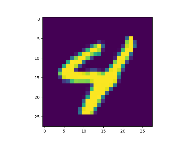
Experiments: MNIST

Now that we have the model, we can try it out on some MNIST experiments. For these experiments we linearize MNIST and just treat each image as a sequence of pixels.

The first experiments we ran were on MNIST classification. While not in theory a hard problem, treating MNIST as a linear sequence classification task is a bit strange. However in practice, the model with $H=256$ and four layers seems to get up near 99% right away.

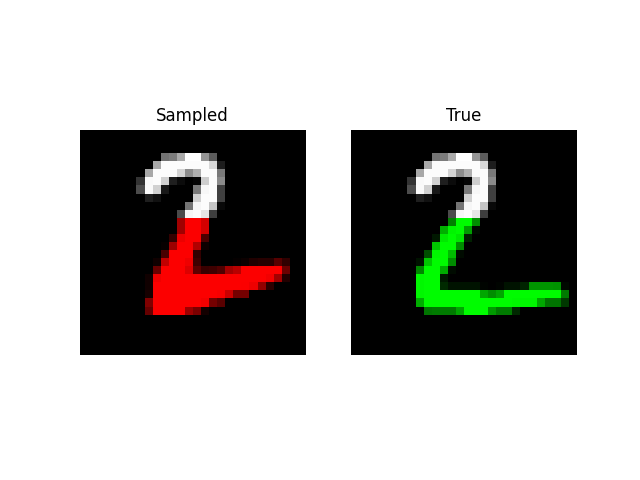
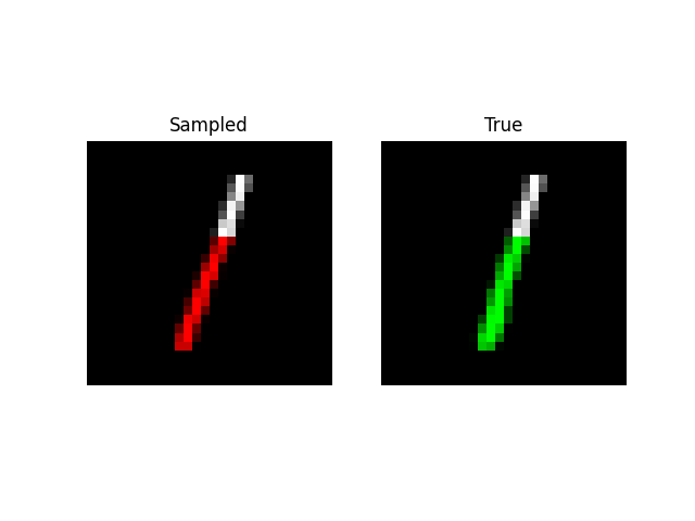
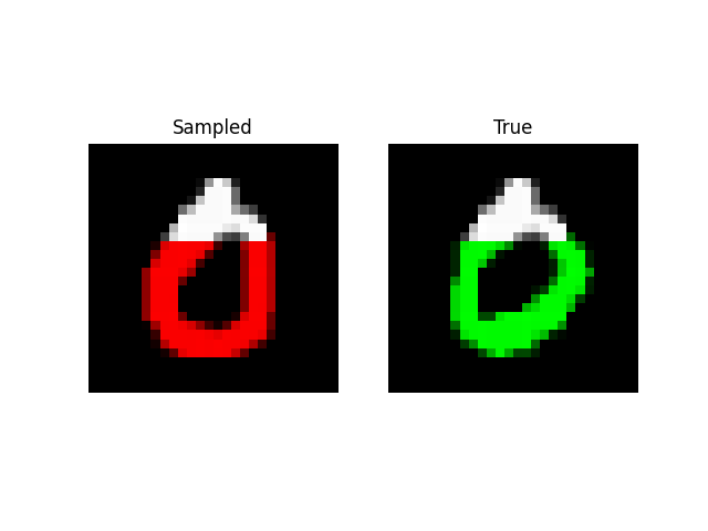
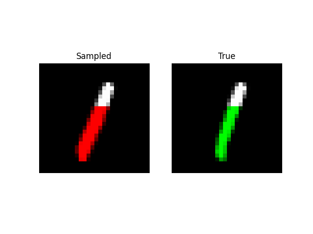
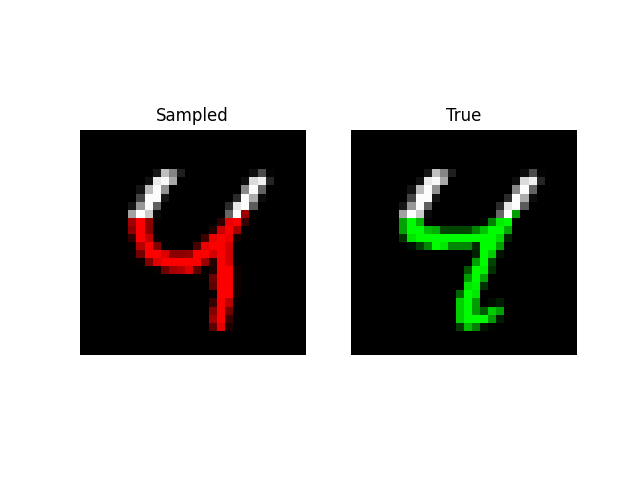
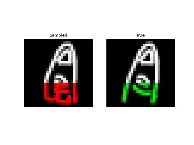
A more visually interesting task is generating MNIST digits, by predicting entire sequences of pixels! Here, we simply feed in a sequence of pixels into the model and have it predict the next one like language modeling. With a little tweaking, we are able to get the model to an NLL of 0.52 on this task with size 512 and 6 layers (~2m parameters).

The metric usually used for this task is bits per dimension which is NLL in base 2 for MNIST. A score of 0.52 is ~0.76 BPD which is near PixelCNN++.

We can also do prefix-samples – given the first 300 pixels, try to complete the image. S4 is on the left, true on the right.

def sample_mnist_prefix(path, model, length):
    import matplotlib.pyplot as plt
    import numpy as onp
    from .data import Datasets

    BATCH = 32
    START = 300
    start = np.zeros((BATCH, length, 1))
    params, prime, init_cache = init_from_checkpoint(model, path, start[:, :-1])

    _, testloader, _, _, _ = Datasets["mnist"](bsz=BATCH)
    it = iter(testloader)
    for j, im in enumerate(it):
        image = im[0].numpy()

        cur = onp.array(image)
        cur[:, START + 1 :, 0] = 0
        cur = np.array(cur)

        # Cache the first `start` inputs.
        out, vars = model.apply(
            {"params": params, "prime": prime, "cache": init_cache},
            cur[:, np.arange(0, START)],
            mutable=["cache"],
        )
        cache = vars["cache"].unfreeze()
        out = sample(model, params, prime, cache, cur, START, length - 1, rng)
        print(j)

        # Visualization
        out = out.reshape(BATCH, 28, 28)
        final = onp.zeros((BATCH, 28, 28, 3))
        final2 = onp.zeros((BATCH, 28, 28, 3))
        final[:, :, :, 0] = out
        f = final.reshape(BATCH, 28 * 28, 3)
        i = image.reshape(BATCH, 28 * 28)
        f[:, :START, 1] = i[:, :START]
        f[:, :START, 2] = i[:, :START]
        f = final2.reshape(BATCH, 28 * 28, 3)
        f[:, :, 1] = i
        f[:, :START, 0] = i[:, :START]
        f[:, :START, 2] = i[:, :START]
        for k in range(BATCH):
            fig, (ax1, ax2) = plt.subplots(ncols=2)
            ax1.set_title("Sampled")
            ax1.imshow(final[k] / 256.0)
            ax2.set_title("True")
            ax1.axis("off")
            ax2.axis("off")
            ax2.imshow(final2[k] / 256.0)
            fig.savefig("im%d.%d.png" % (j, k))
            print(j)

Experiments: QuickDraw

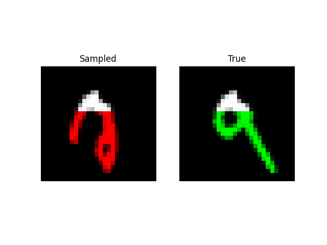
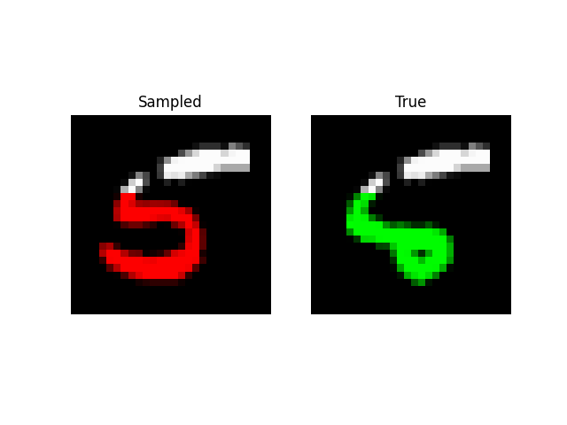
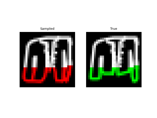
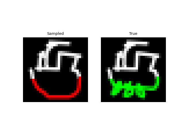
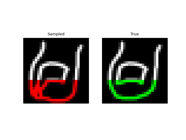
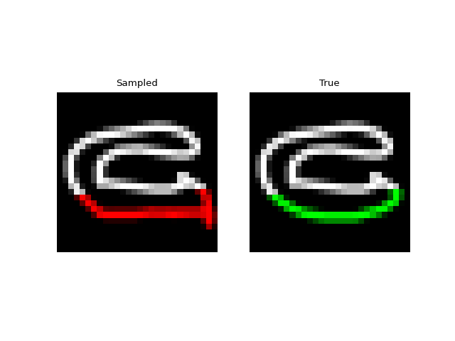
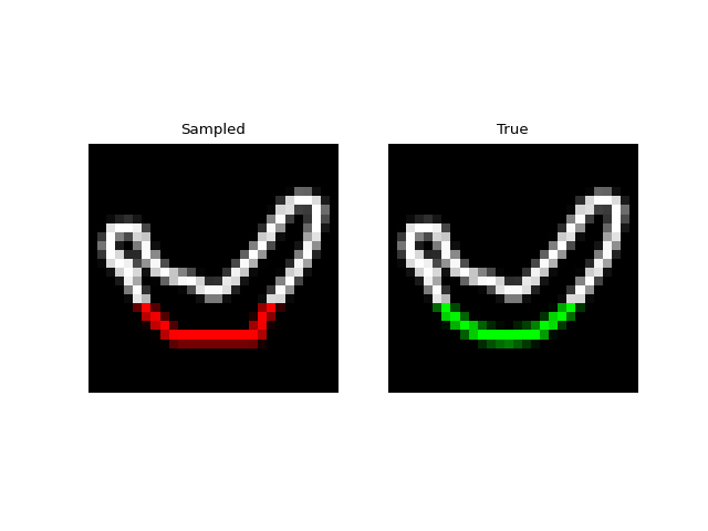
Next we tried training a model to generate drawings. For this we used the QuickDraw dataset. The dataset includes a version of the dataset downsampled to MNIST size so we can use roughly the same model as above. The dataset is much larger though (5M images) and more complex. We only trained for 1 epoch with a $H=256$, 4 layer model. Still, the approach was able to generate relatively coherent completions. These are prefix samples with 500 pixels given.

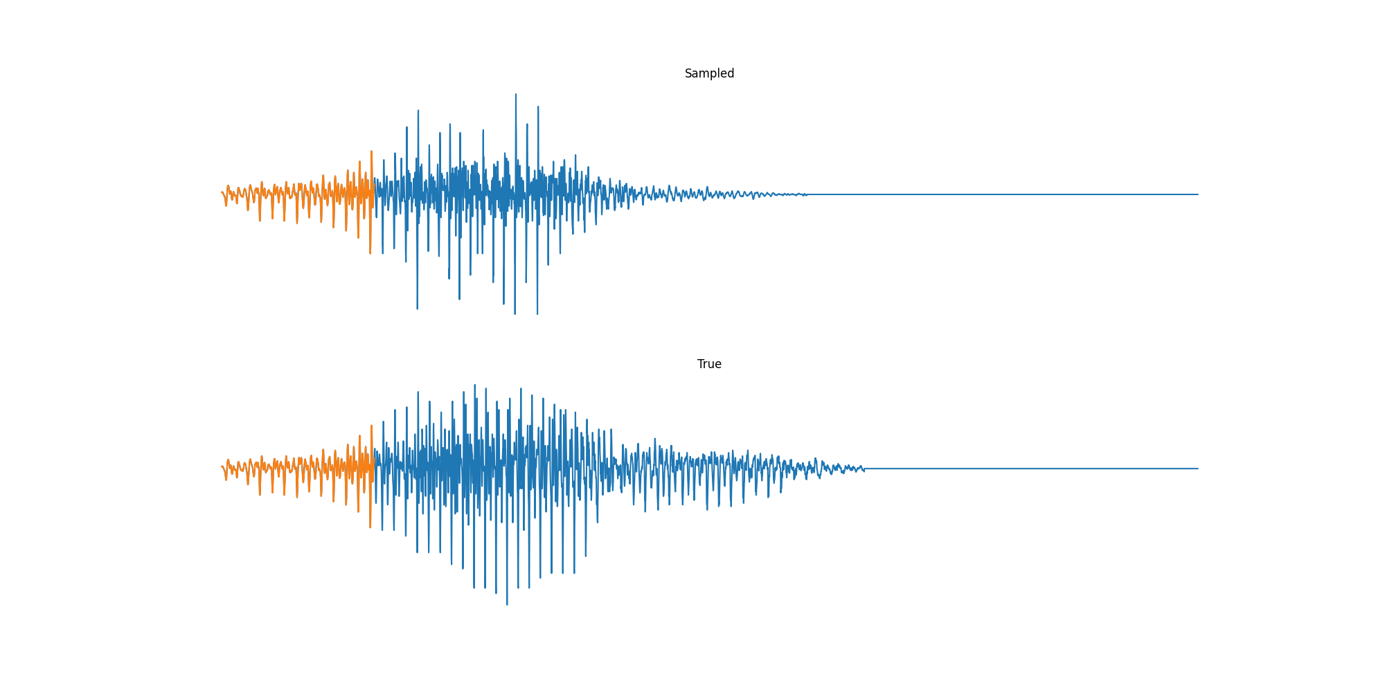
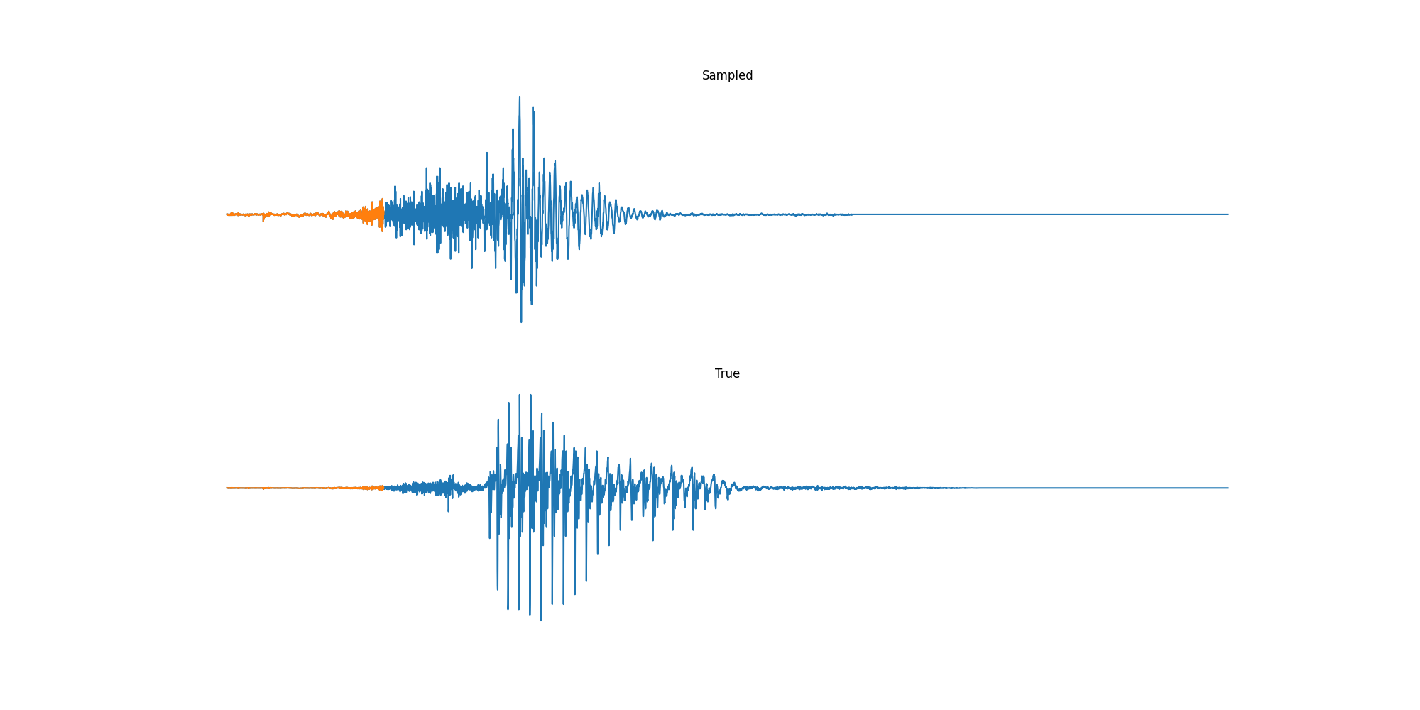
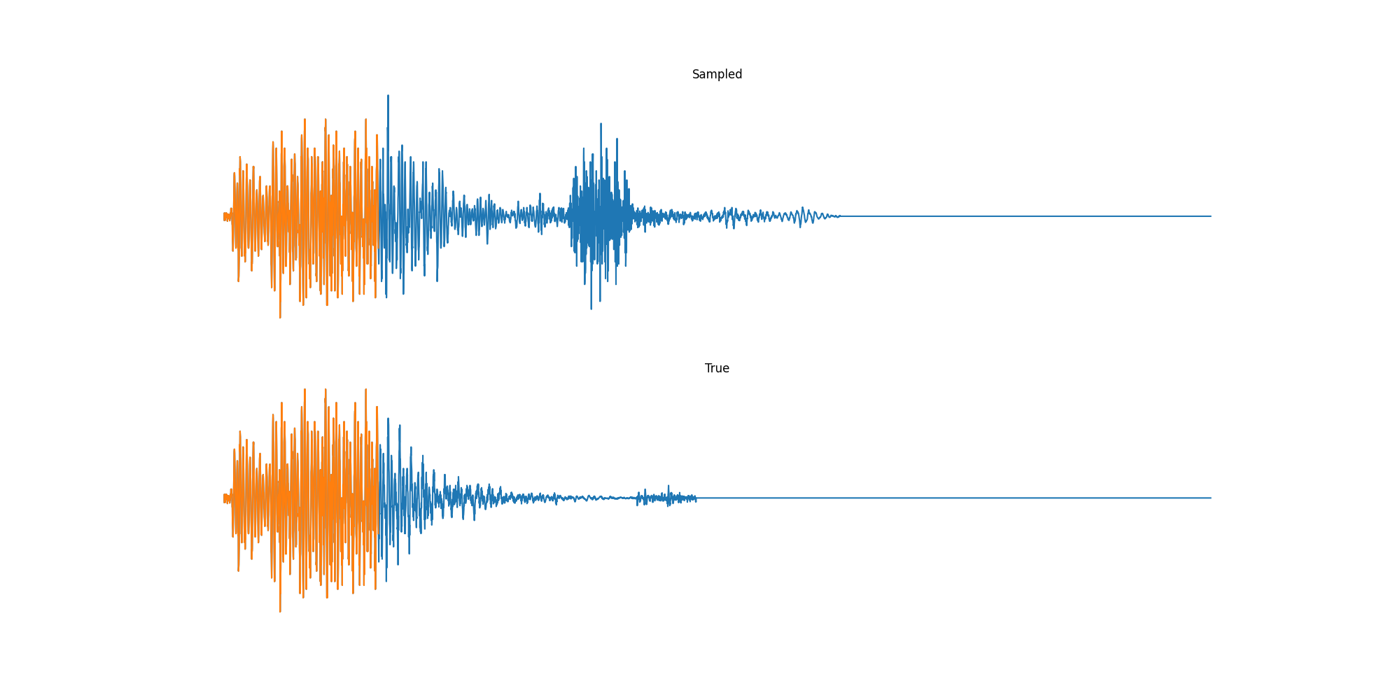
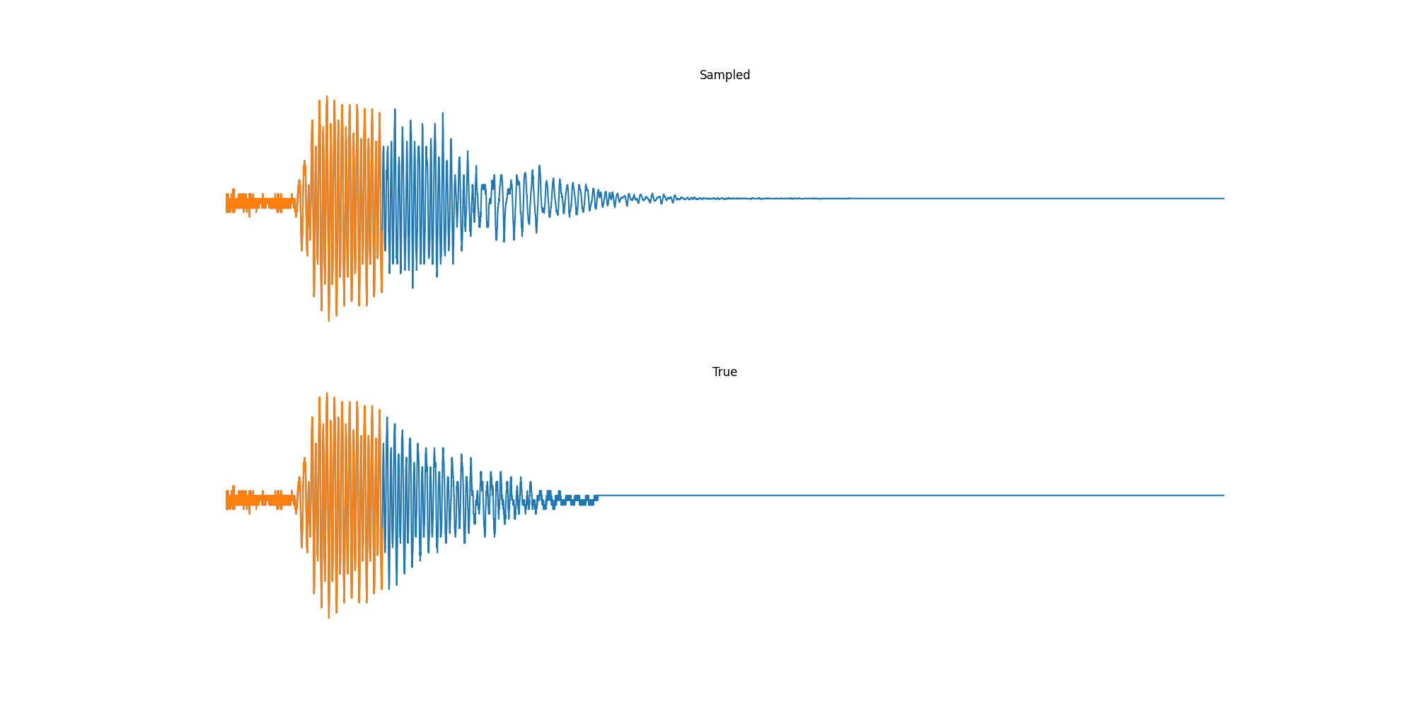
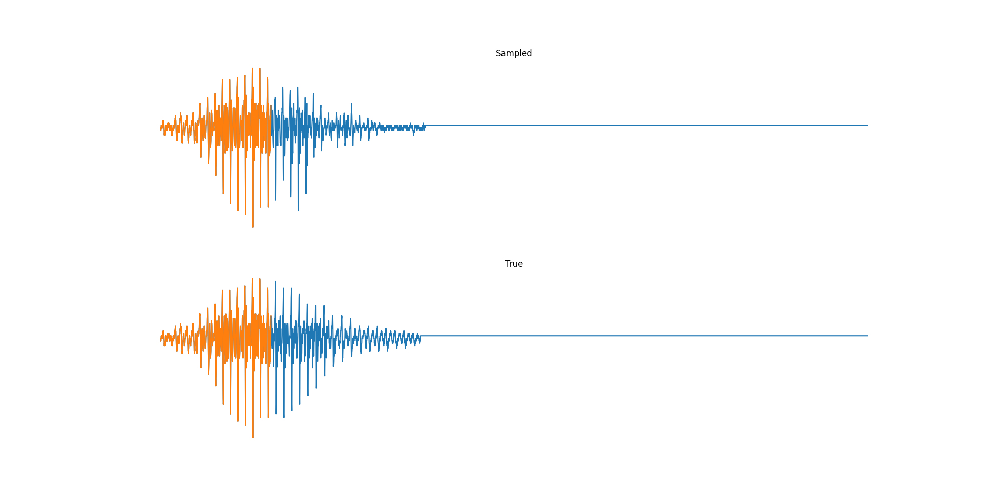
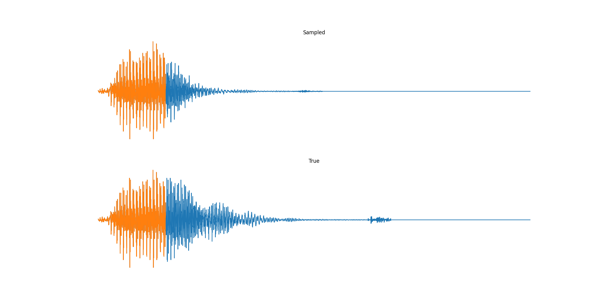
Experiments: Spoken Digits

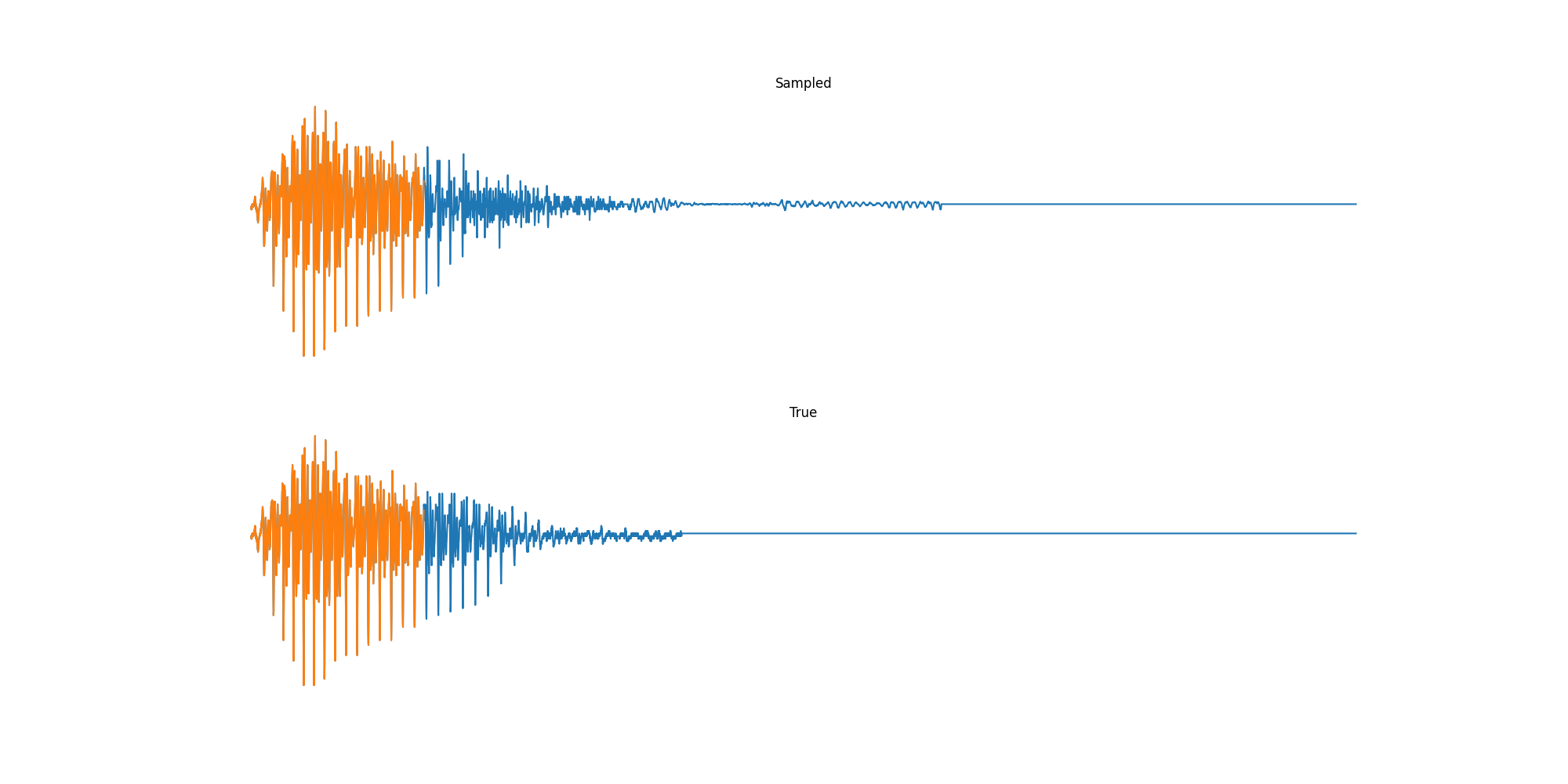
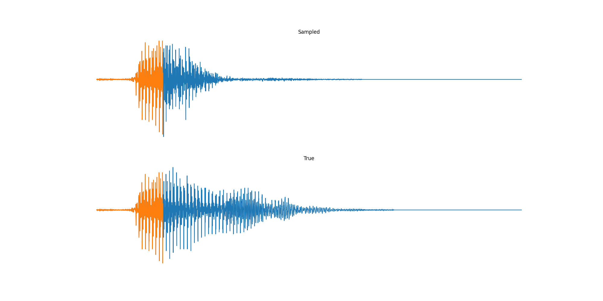
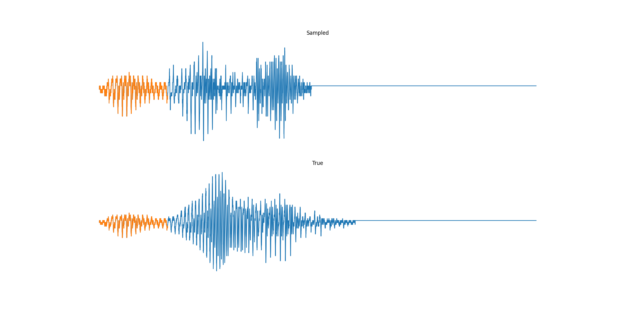
Finally we played with modeling sound waves directly. For these, we use the Free Spoken Digits Datasets an MNIST like dataset of various speakers reading off digits. We first trained a classification model and found that the approach was able to reach $97\%$ accuracy just from the raw soundwave. Next we trained a generation model to produce the sound wave directly. With $H=512$ the model seems to pick up the data relatively well. This dataset only has around 3000 examples, but the model can produce reasonably good (cherry-picked) continuations. Note these sequences are 6400 steps long at an 8kHz sampling rate, discretized to 256 classes with Mu Law Encoding.

Our full code base contains more examples and infrastructure for training models for generations and classification.

Conclusion

Putting together this post inspired lots of thoughts about future work in this area. One obvious conclusion is that long-range models have all sorts of future applications from acoustic modeling to genomic sequences to trajectories (not to mention our shared area of NLP). Another is some surprise that linear models can be so effective here, while also opening up a range of efficient techniques. Finally from a practical level, the transformations in JAX make it really nice to implement complex models like this in a very concise way (~200 LoC), with similar efficiency and performance!

We end by thanking the authors Albert Gu and Karan Goel, who were super helpful in putting this together, and pointing you again to their paper and codebase. We’re also grateful for Conner Vercellino and Laurel Orr for providing helpful feedback on this post.

/ Cheers – Sasha & Sidd