Looking at the Performer from a Hopfield Point of View
25 Mar 2022 | deep-learning hopfield-networks associative-memory attention transformerThe Performer blog post can be used as a proper explanation of the paper.
In this blog post, we look at the Performer from a Hopfield Network point of view and relate aspects of the Performer architecture to findings in the field of associative memories and Hopfield Networks. This blog post sheds light on the Performer from three different directions:
- Performers resemble classical Hopfield Networks. Recently, it was shown that the update rule of modern continuous Hopfield Networks is the attention of the Transformer. We now show that generalized kernelizable attention of the Performer resembles the update rule of classical Hopfield Networks.
- Sparseness increases memory capacity. We point out that sparseness considerably increases the memory capacity in classical Hopfield Networks and associative memories, and discuss how sparseness is achieved by the Performer.
- Performer normalization relates to the activation function of continuous Hopfield Networks. We correlate the normalization term $ \widehat{D}^{-1} $ of the Performer with activation functions of classical continuous Hopfield Networks.
This blog post is structured as follows: We start with a short review of classical Hopfield Networks, then interpret generalized kernelizable attention of the Performer as one-step update of a classical Hopfield Network (discrete and continuous), and discuss sparseness and normalization of the Performer. Finally, we show an exemplary implementation of a continuous classical Hopfield Network for illustrative purposes. With this blog post we aim at contributing to a better understanding of Transformer models. This blog post loosely builds on the paper Hopfield Networks is All You Need and the corresponding blog post.
Classical Hopfield Networks
This part is taken from the Hopfield Networks is All You Need blog post. A very good overview of Hopfield Networks can be found here.
Binary (Polar) Classical Hopfield Networks
The simplest associative memory is just a sum of outer products of the $ N $ patterns $ \{\mathbf{x}_{i}\}_{i=1}^{N} $ that we want to store (Hebbian learning rule). In classical Hopfield Networks these patterns are polar or binary, i.e. $ \boldsymbol{x}_{i} \in \{ -1,1 \}^{d} $ or $ \boldsymbol{x}_{i} \in \{ 0,1 \}^{d} $, respectively, where $ d $ is the length of the patterns. The corresponding weight matrix $ \boldsymbol{W} $ for $ \boldsymbol{X}=(\boldsymbol{x}_{1},\dotsc,\boldsymbol{x}_{N})$ is:
\[\begin{equation} \boldsymbol{W} = \boldsymbol{X}\boldsymbol{X}^{T} . \tag{1} \end{equation}\]The weight matrix $ \boldsymbol{W} $ stores the patterns, from which a pattern is retrieved starting with a state pattern $ \boldsymbol{\xi} $.
The basic synchronous update rule is to repeatedly multiply the state pattern $ \boldsymbol{\xi} $ with the weight matrix $ \boldsymbol{W} $, subtract the bias and take the sign:
\[\begin{equation} \boldsymbol{\xi}^{t+1} = \text{sgn}(\boldsymbol{W}\boldsymbol{\xi}^{t} - \boldsymbol{b}) \ , \tag{2} \label{eq:restorage} \end{equation}\]where $ \boldsymbol{b} \in \mathbb{R}^{d} $ is a bias vector, which can be interpreted as a threshold for every component. The asynchronous update rule performs this update only for one component of $ \boldsymbol{\xi} $ and then selects the next component. Convergence is reached if $ \boldsymbol{\xi}^{t+1} = \boldsymbol{\xi}^{t} $.
The asynchronous version of the update rule of Eq. \eqref{eq:restorage} minimizes the energy function $ \text{E} $:
\[\newcommand{\subscript}[2]{#1_{#2}} \begin{equation} \text{E} = -\frac{1}{2}\boldsymbol{\xi}^{T} \boldsymbol{W} \boldsymbol{\xi} + \boldsymbol{\xi}^{T}\boldsymbol{b} = -\frac{1}{2} \subscript{\sum}{i=1}^{d}\subscript{\sum}{j=1}^{d} \subscript{w}{ij}\subscript{\xi}{i}\xi_{j} + \subscript{\sum}{i=1}^{d} \subscript{b}{i}\subscript{\xi}{i} \ . \tag{3} \label{eq:energyHopfield} \end{equation}\]As derived in the papers of Bruck, Goles-Chacc et al. and the original Hopfield paper, the convergence properties are dependent on the structure of the weight matrix $ \boldsymbol{W} $ and the method by which the nodes are updated:
- For asynchronous updates with $ w_{ii} \geq 0 $ and $ w_{ij} = w_{ji} $, the updates converge to a stable state.
- For synchronous updates with $ w_{ij} = w_{ji} $, the updates converge to a stable state or a limit cycle of length 2.
For the asynchronous update rule and symmetric weights, $ \text{E}(\boldsymbol{\xi}^{t+1}) \leq \text{E}(\boldsymbol{\xi}^{t}) $ holds. When $ \text{E}(\boldsymbol{\xi}^{t+1}) = \text{E}(\boldsymbol{\xi}^{t}) $ for the update of every component of $ \boldsymbol{\xi}^{t} $, a local minimum in $ \text{E} $ is reached. For multiple, say $ M $, state patterns summarized in a matrix $ \boldsymbol{Q}=(\boldsymbol{\xi}_{1},\dotsc,\boldsymbol{\xi}_{M}) $ and $ \boldsymbol{b}=0 $, the update rule reads
\[\begin{equation} \widetilde{\boldsymbol{Q}} = \text{sgn}(\boldsymbol{W}\boldsymbol{Q}) \ . \tag{4} \label{eq:updateHopfield} \end{equation}\]An illustration of the pattern retrieval mechanism can be found in the Hopfield Networks is All You Need blog post.

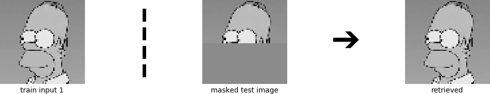
The weight matrix $ \boldsymbol{W} $ is the outer product of this black and white image $ \boldsymbol{x}_{\text{Homer}} $:
\[\newcommand{\subscript}[2]{#1_{#2}} \begin{equation} \boldsymbol{W} = \subscript{\boldsymbol{x}}{\text{Homer}}^{\text{ }} \subscript{\boldsymbol{x}}{\text{Homer}}^T \ , \qquad \subscript{\boldsymbol{x}}{\text{Homer}}^{\text{ }} \in \{ -1,1\}^{d} \ , \tag{5} \label{eq:weightMatrix} \end{equation}\]where for this example $ d = 64 \times 64 $. It takes one update until the original image is restored.

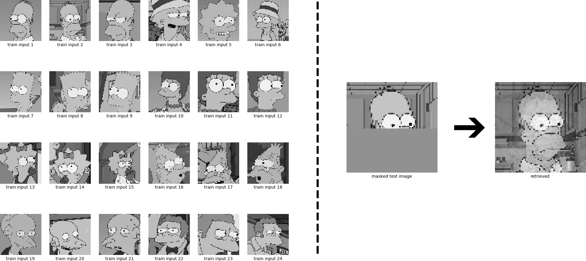
What happens if we store more than one pattern? The weight matrix is then built from the sum of outer product of six stored patterns:
\[\newcommand{\subscript}[2]{#1_{#2}} \begin{equation} \boldsymbol{W} = \sum_{i=1}^{6} \subscript{\boldsymbol{x}}{i}^{\text{ }} \subscript{\boldsymbol{x}}{i}^{T} \ , \qquad \subscript{\boldsymbol{x}}{i} \in \{ -1,1\}^d \ . \tag{6} \end{equation}\]The six stored patterns refer to the six input images:

The example patterns are correlated, and therefore the retrieval has errors.
Continuous Classical Hopfield Networks
The Performer works with continuous activations while the Hopfield Network is binary. However, also continuous versions of Hopfield Networks have been proposed. The energy function of continuous classical Hopfield Networks is treated by Hopfield in 1984, Koiran in 1994 and Wang in 1998. For continuous classical Hopfield Networks the energy function of Eq. \eqref{eq:energyHopfield} is expanded to:
\[\newcommand{\subscript}[2]{#1_{#2}} \begin{equation} \text{E} (\boldsymbol{\xi}) = -\frac{1}{2}\boldsymbol{\xi}^{T} \boldsymbol{W} \boldsymbol{\xi} + \boldsymbol{\xi}^{T}\boldsymbol{b} + \subscript{\sum}{i=1}^{d} \subscript{\int}0^{\xi[i]} f^{-1}(y) \ dy \ , \tag{7} \label{eq:energyHopfieldContinuous} \end{equation}\]where $ \xi[i] $ denotes the $ i $-th component of $ \boldsymbol{\xi} $.
In Hopfield’s paper and in an informative Scholarpedia article, it is shown that the energy function $ \text{E} (\boldsymbol{\xi}) $ of Eq. \eqref{eq:energyHopfieldContinuous} is a Lyapunov function of the (continuous) dynamics of $ \boldsymbol{\xi} $. In literature, update rules are derived via the underlying ordinary differential equation of the Lyapunov function (Hopfield, Koiran, Scholarpedia article). Here, the update rule is derived by applying the Concave-Convex-Procedure (CCCP) described by Yuille and Rangarajan on the energy function of Eq. \eqref{eq:energyHopfieldContinuous}:
- The total energy $ \text{E}(\boldsymbol{\xi}) $ is split into a convex and a concave term: $ \newcommand{\subscript}[2]{#1_{#2}} \text{E}(\boldsymbol{\xi}) = \subscript{\text{E}}{1}(\boldsymbol{\xi}) + \subscript{\text{E}}{2}(\boldsymbol{\xi}) $
- The term $ \newcommand{\subscript}[2]{#1_{#2}} \subscript{\sum}{i=1}^{d} \subscript{\int}{0}^{\xi[i]} f^{-1}(y) \ dy = \subscript{\text{E}}{1}(\boldsymbol{\xi}) $ is convex. We will later see which conditions are sufficient for $ \newcommand{\subscript}[2]{#1_{#2}} \subscript{\text{E}}{1}(\boldsymbol{\xi}) $ to be convex.
- The term $ \newcommand{\subscript}[2]{#1_{#2}} -\frac{1}{2}\boldsymbol{\xi}^{T} \boldsymbol{W} \boldsymbol{\xi} + \boldsymbol{\xi}^{T}\boldsymbol{b} = \subscript{\text{E}}{2}(\boldsymbol{\xi}) $ is concave. Since $ \boldsymbol{W} $ is positive semi-definite (every matrix which can be written as sum of outer products is), $ \frac{1}{2}\boldsymbol{\xi}^{T} \boldsymbol{W} \boldsymbol{\xi} $ is convex.
- The CCCP applied to $ \text{E} $ is:
In order for $ \text{E}_1(\boldsymbol{\xi}) $ to be convex, it is sufficient to ensure that $ f(y) $ is strictly increasing. To see this, the argument is as follows: If $ f(y) $ is stricly increasing, then also $ f^{-1}(y) $ is strictly increasing. Consequently, the derivative of $ f^{-1}(y) $ is larger than zero and therefore
\[\newcommand{\subscript}[2]{#1_{#2}} \begin{equation} \frac{\partial^{2} \subscript{\text{E}}{1}(\boldsymbol{\xi})}{\partial \xi[i] \partial \xi[j]}= \begin{cases} (f^{-1})'(\xi[i])>0 & \text{ if } i=j \\ 0 & \, \text{else}\end{cases}. \tag{11} \end{equation}\]This implies that the Hessian of $ \text{E}_1(\boldsymbol{\xi}) $ is a diagonal matrix with strictly positive diagonal elements, thus it is positive definite and therefore $ \text{E}_1(\boldsymbol{\xi}) $ is convex.
Many activation functions fulfill these requirements. In the literature, usually the tangens hyperbolicus or sigmoid function is used.
If we now set $ f(y) = \tanh $, we can rewrite Eq. \eqref{eq:updateCpp3} as:
\[\newcommand{\subscript}[2]{#1_{#2}} \begin{align} \tanh^{-1}(\boldsymbol{\xi}^{t+1}) &= \boldsymbol{W}\boldsymbol{\xi}^{t} - \boldsymbol{b} \tag{12} \label{eq:updateCpp4} \\[10px] \boldsymbol{\xi}^{t+1} &= \tanh \left(\boldsymbol{W}\boldsymbol{\xi}^{t} - \boldsymbol{b} \right) \ . \tag{13} \label{eq:updateCpp5} \end{align}\]Note that by abuse of notation we apply $ f $ elementwise here. This now looks very familiar to a one-layer neural network. Similarly as in Eq. \eqref{eq:updateHopfield}, for multiple, say $ M $, state patterns summarized in a matrix $ \boldsymbol{Q}=(\boldsymbol{\xi}_1,\dotsc,\boldsymbol{\xi}_M) $ and $ \boldsymbol{b}=0 $, the update rule reads
\[\begin{equation} \widetilde{\boldsymbol{Q}} = \tanh(\boldsymbol{W}\boldsymbol{Q}) \ . \tag{14} \label{eq:updateHopfieldContinuous} \end{equation}\]Performer Attention Resembles Update of Classical Hopfield Networks
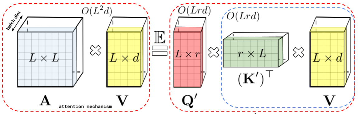
The following image is taken from the Rethinking Attention with Performers paper. On the left, the Transformer self-attention mechanism introduced in the paper Attention is All You Need is shown. The complexity of the Transformer self-attention is quadratic with respect to the number of input tokens $ L $. On the right, the linear attention framework of the Performer is shown. The linear generalized kernelizable attention is implemented via the so-called FAVOR+ (Fast Attention Via positive Orthogonal Random features) mechanism.
Let’s start by writing down the Transformer self-attention $ \boldsymbol{Z} $ for $ L $ tokens, hidden dimension $ d $, token input dimension $ i $:
\[\newcommand{\subscript}[2]{#1_{#2}} \begin{equation} \boldsymbol{Z} = \text{softmax} \left(\frac{1}{\sqrt{\subscript{d}{K}}} \boldsymbol{Q}\boldsymbol{K}^{T} \right) \boldsymbol{V} \ , \tag{15} \end{equation}\]where the dimensions of the involved matrices are the following:
\[\newcommand{\subscript}[2]{#1_{#2}} \begin{alignat}{5} & && &&\boldsymbol{Z} &&\in \mathbb{R}^{L \times d} \ , \tag{16} \\ &\boldsymbol{Q} &&= \subscript{\boldsymbol{XW}}{Q} \ , \quad &&\boldsymbol{Q} &&\in \mathbb{R}^{L \times d} \ , \boldsymbol{X} &&\in \mathbb{R}^{L \times i} \ , \subscript{\boldsymbol{W}}{Q} &&\in \mathbb{R}^{i \times d} \ , \tag{17} \\ &\boldsymbol{K}^{T} &&= \subscript{\boldsymbol{W}}{K}^{T} \boldsymbol{X}^{T} \ , \quad &&\boldsymbol{K}^{T} &&\in \mathbb{R}^{d \times L} \ , \subscript{\boldsymbol{W}}{K}^{T} &&\in \mathbb{R}^{d \times i} \ , \boldsymbol{X}^{T} &&\in \mathbb{R}^{i \times L} \ , \tag{18} \\ &\boldsymbol{V} &&= \subscript{\boldsymbol{XW}}{V} \ , \quad &&\boldsymbol{V} &&\in \mathbb{R}^{L \times d} \ , \boldsymbol{X} &&\in \mathbb{R}^{L \times i} \ , \subscript{\boldsymbol{W}}{V} &&\in \mathbb{R}^{i \times d} \ . \tag{19} \end{alignat}\]$ d_{K} $ denotes some normalization constant, often it is set to $ d_K=d $.
In the Performer paper, the FAVOR+ mechanism is introduced and the Transformer self-attention is substituted by generalized kernelizable attention, whose complexity scales linearly with the number of input tokens $ L $. The idea of the Performer is to decompose the attention matrix into a matrix product:
\[\newcommand{\subscript}[2]{#1_{#2}} \begin{equation} \subscript{\boldsymbol{A}}{\text{Perf}} = \widehat{\boldsymbol{D}}^{-1} \boldsymbol{Q'} \boldsymbol{K'}^{T} \ , \tag{21} \end{equation}\]where $ \boldsymbol{Q’} $ and $ \boldsymbol{K’} $ can be directly computed from the queries $ \boldsymbol{Q} $ and the keys $ \boldsymbol{K} $ using a kernel function $ \phi: \mathbb{R}^{d} \rightarrow \mathbb{R}^{r} $, which maps:
\[\begin{alignat}{3} & \boldsymbol{Q} &&\rightarrow \boldsymbol{Q'} \ , \quad &&\boldsymbol{Q'} &&\in \mathbb{R}^{L \times r} \ , \tag{22} \\ & \boldsymbol{K}^{T} &&\rightarrow \boldsymbol{K'}^{T} \ , \quad &&\boldsymbol{K'}^{T} &&\in \mathbb{R}^{r \times L} \ . \tag{23} \end{alignat}\]Consequently, the generalized kernelizable attention $ \boldsymbol{Z’} $ reads
\[\begin{equation} \boldsymbol{Z'} = \widehat{\boldsymbol{D}}^{-1} \left( \boldsymbol{Q'} \left(\boldsymbol{K'}^{T} \boldsymbol{V} \right) \right) \ , \tag{24} \end{equation} \label{eq:performerAttention}\]where $ \widehat{\boldsymbol{D}}^{-1} = \text{diag}\left(\boldsymbol{Q’}\boldsymbol{K’}^{T}\boldsymbol{1}_L \right) $, and the dimensions of the involved matrices are the following:
\[\begin{alignat}{2} & &&\boldsymbol{Z'} &&\in \mathbb{R}^{L \times d} \ , \tag{25} \\ & &&\boldsymbol{Q'} &&\in \mathbb{R}^{L \times r} \ , \tag{26} \\ & &&\boldsymbol{K'}^{T} &&\in \mathbb{R}^{r \times L} \ , \tag{27} \\ & &&\boldsymbol{V} &&\in \mathbb{R}^{L \times d} \ . \tag{28} & &&\end{alignat}\]The matrix product $ \boldsymbol{K’}^{T} \boldsymbol{V} = \boldsymbol{W} $ is the sum of outer products and has the dimension $ \boldsymbol{W} \in \mathbb{R}^{r \times d} $. For $ r = d $, we have
\[\begin{equation} \widetilde{\boldsymbol{Q}}' = \boldsymbol{Q'} \boldsymbol{W} \ , \tag{29} \label{eq:performerAttention2} \end{equation}\]which resembles the transposed one-step update of classical binary (polar) and continuous Hopfield Networks introduced for pattern retrieval in Eq. \eqref{eq:updateHopfield} and Eq. \eqref{eq:updateHopfieldContinuous}, respectively.
Both the mapping $ \phi: \mathbb{R}^{d} \rightarrow \mathbb{R}^{r} $ of Eq. \eqref{eq:performerAttention} and the normalization $ \widehat{\boldsymbol{D}}^{-1} $ of Eq. \eqref{eq:performerAttention} play an important role. This is discussed in the next paragraph.
The Performer Related to Classical Hopfield Networks
We now relate the Performer to known facts from the field of Hopfield Networks and associative memories, namely sparseness, one-step update and storage capacity. We further look at continuous classical Hopfield Networks and investigate the generalized kernelizable attention of the Performer, especially by looking at the mapping $ \phi: \mathbb{R}^{d} \rightarrow \mathbb{R}^{r} $ and the normalization $ \widehat{\boldsymbol{D}}^{-1} $ of Eq. \eqref{eq:performerAttention}.
About sparseness, one-step update and storage capacity
One obvious difference between the update of classical Hopfield Networks stated in Eq. \eqref{eq:updateHopfield} and the matrix product $ \boldsymbol{Q’} \left(\boldsymbol{K’}^{T} \boldsymbol{V} \right) = \boldsymbol{Q’} \boldsymbol{W} $ of the generalized kernelizable attention of Eq. \eqref{eq:performerAttention2} is that the classical Hopfield Network update can be iteratively applied multiple times, whereas the matrix product $ \boldsymbol{Q’} \boldsymbol{W} $ is applied only once. One-step update for classical Hopfield Networks was e.g. investigated in Schwenker et al. and in Palm. The storage capacity of classical binary Hopfield Networks for fixed-point retrieval of patterns (multiple updates) with a small percentage of errors is $ C \cong 0.14d $. In Schwenker et al., it is shown that for auto-association one-step retrieval achieves nearly the same capacity values as fixed-point retrieval does. Furthermore, in Palm it is stated that using sparse patterns turns out to achieve much higher capacity values ($ C=0.72d $ for one-step retrieval, which is a factor 5 higher than the classical network capacity $ C=0.14d $). In Tsodyks et al., the storage capacity is even found to increase with $ C(p) \sim \frac{1}{p|\ln p|}d $, where $ p $ is the percentage of non-zero weights. An overview of the storage capacities can be found in Knoblauch et al., storage capacities in classical Hopfield Networks are also discussed in the blog Hopfield Networks is All You Need.
To summarize: Sparse patterns yield very large storage capacities, also for one-step retrieval. Below we have a closer look at the mapping $ \phi: \mathbb{R}^{d} \rightarrow \mathbb{R}^{r} $ in the Rethinking Attention with Performers paper and relate the choices of the paper with this statement.
About the mapping $ \phi $ and about the normalization $ \widehat{\boldsymbol{D}}^{-1} $
In the paper Rethinking Attention with Performers, a kernel function $ \phi: \mathbb{R}^{d} \rightarrow \mathbb{R}^{r} $ maps $ \boldsymbol{Q} \rightarrow \boldsymbol{Q’} $ and $ \boldsymbol{K}^{T} \rightarrow \boldsymbol{K’}^{T} $. The kernel function $ \phi $ is of the form:
\[\newcommand{\subscript}[2]{#1_{#2}} \begin{equation} \phi(\boldsymbol{z}) = \frac{h(\boldsymbol{z})}{\sqrt{r}} \left(\subscript{f}{1}(\subscript{\boldsymbol{w}}{1}^{T} \boldsymbol{z}),\dotsc,\subscript{f}{1}(\subscript{\boldsymbol{w}}{m}^{T}\boldsymbol{z}),\dotsc, \subscript{f}{l}(\subscript{\boldsymbol{w}}{1}^{T}\boldsymbol{z}),\dotsc,\subscript{f}{l}( \subscript{\boldsymbol{w}}{m}^{T}\boldsymbol{z}) \right)\ , \tag{30} \label{eq:kernelFunction} \end{equation}\]where $ \boldsymbol{z} $ are the row vectors of $ \boldsymbol{Q} $ and $ \boldsymbol{K} $ (i.e. column vectors of $ \boldsymbol{K}^{T} $), $ f_{1},\dotsc,f_{l} $ are functions that map from $ \mathbb{R}\rightarrow\mathbb{R} $, $ h $ is a function that maps from $ \mathbb{R}^{d} \rightarrow \mathbb{R} $, and $ \boldsymbol{w}_{1},\dotsc,\boldsymbol{w}_{m} \overset{iid}{\sim} \mathcal{D} $ are vectors from some distribution $ \mathcal{D}\in \mathcal{P}(\mathbb{R})^{d} $. It also immediately follows that $ r=l \cdot m $. In the paper, it turns out to work best if $ m=r $, $ l=1 $, $ \boldsymbol{w}_{1},\dotsc,\boldsymbol{w}_{r} $ are orthogonal random feature maps, and the ReLU function is used for $ f_1 $.
Continuous Hopfield Networks for Illustrative Purposes
In this last part of the blog, we look at some illustrative examples:
- Continuous classical Hopfield Networks
- Sparse continuous classical Hopfield Networks
- Modern continuous Hopfield Networks
- Sparse modern continuous Hopfield Networks
- Performer Networks
- Sparse Performer Networks
Continuous Classical Hopfield Networks
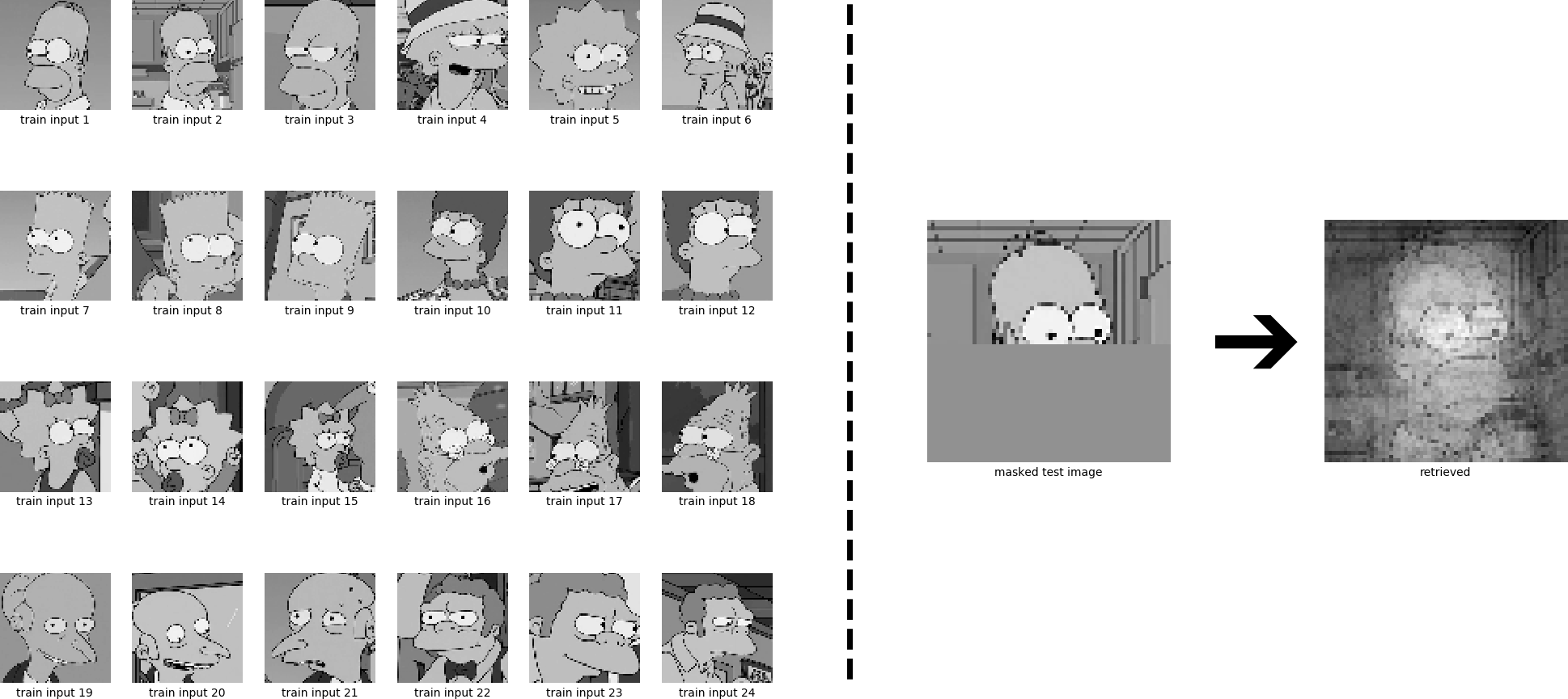
We first implement a continuous classical Hopfield Network, and we are going to retrieve a continuous Homer ($ \boldsymbol{\xi} $) out of many continuous stored patterns $ \boldsymbol{X}=(\boldsymbol{x}_{1},\dotsc,\boldsymbol{x}_{N}) $ using Eq. \eqref{eq:updateCpp5}. Instead of polar patterns, i.e. $ \boldsymbol{x}_{i} \in \{ -1, 1\}^{d} $ where $ d $ is the length of the patterns, patterns are now continuous, i.e. $ \boldsymbol{x}_{i} \in \left[ -1, 1\right]^{d} $.
We start again with the retrieval of only one stored pattern, which is not a too hard job.
The next task is again a retrieval out of six stored patterns, which already does not work any more.

Sparse Continuous Classical Hopfield Networks
We will now exploit the insight from above, namely that sparse patterns yield very large storage capacities. Therefore, all components $ \boldsymbol{\xi}[l] > -0.5 $ and all components $ \boldsymbol{x}_{i}[l] > -0.5 $ of $ \boldsymbol{X}^{T} $ are set to zero, giving $ \boldsymbol{\xi}^{\text{ }}_{\text{sparse}} $ and $ \boldsymbol{X}^{T}_{\text{sparse}} $, respectively. The sparse version of Eq. \eqref{eq:updateCpp5} now reads:
\[\newcommand{\subscript}[2]{#1_{#2}} \begin{equation} \boldsymbol{\xi}^{\text{new}} = \tanh \left(\boldsymbol{X}\subscript{\boldsymbol{X}}{\text{sparse}}^{T} \subscript{\boldsymbol{\xi}}{\text{sparse}} \right) \ . \tag{31} \label{eq:updateCpp5Sparse} \end{equation}\]
Pattern retrieval now works for 6 stored patterns, but what about more patterns?
Modern Continuous Hopfield Networks
It seems that a model with larger storage capacity is needed. Recently, Modern Continuous Hopfield Networks for Deep Learning Architectures were introduced in the paper Hopfield Networks is All You Need. It was shown that modern continuous Hopfield Networks can store exponentially (in $ d $) many patterns. To retrieve a pattern $ \boldsymbol{\xi} $, the update rule of modern continuous Hopfield Networks for $ N $ stored patterns $ \boldsymbol{X} = (\boldsymbol{x}_{1},\dotsc,\boldsymbol{x}_{N}) $ reads:
\[\begin{equation} \boldsymbol{\xi}^{\text{new}} = \boldsymbol{X} \text{softmax} (\beta \boldsymbol{X}^{T} \boldsymbol{\xi}) \ , \tag{32} \label{eq:updateModernHopfield} \end{equation}\]where $ \beta $ is the inverse temperature controlling the learning dynamics. We choose the value $ \beta = 25 $, which enables useful pattern retrieval for 6 stored patterns, but fails if 24 patterns are stored. Note that the learning dynamics for $ \beta = 25 $ are different to the ones shown in the Hopfield blog post due to normalization of the patterns.
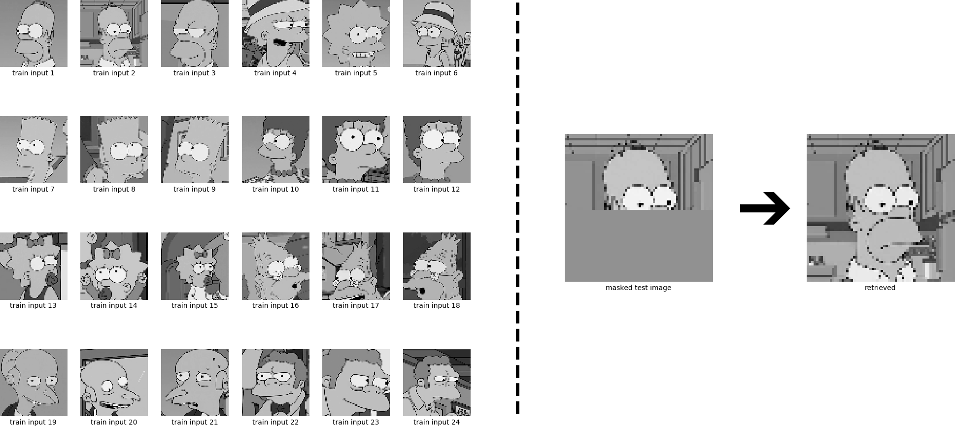
For 6 stored patterns:

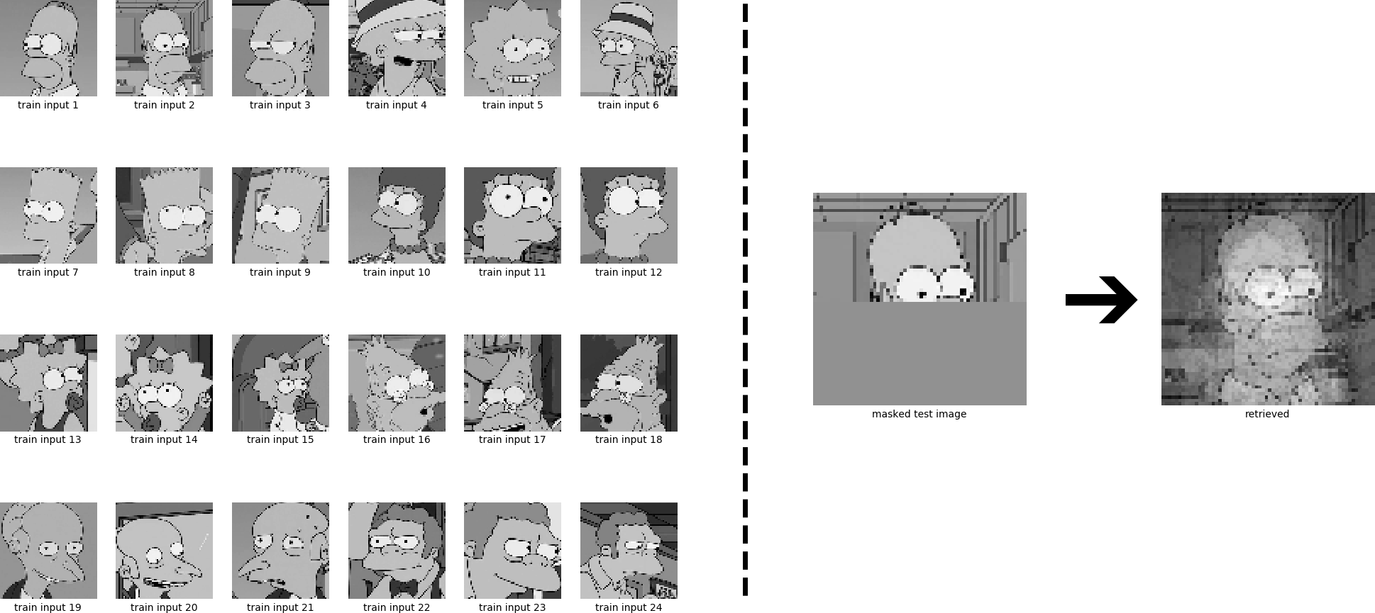
For 24 stored patterns:
Sparse Modern Continuous Hopfield Networks
We will now again exploit the insight from above, namely that sparse patterns yield very large storage capacities. Therefore, in Eq. \eqref{eq:updateModernHopfield} all components $ \boldsymbol{\xi}[l] > -0.5 $ and all components $ \boldsymbol{x}_{i}[l] > -0.5 $ of $ \boldsymbol{X}^{T} $ are set to zero, giving $ \boldsymbol{\xi}_{\text{sparse}}^{\text{ }} $ and $ \boldsymbol{X}^{T}_{\text{sparse}} $, respectively. The sparse version of Eq. \eqref{eq:updateModernHopfield} now reads:
\[\newcommand{\subscript}[2]{#1_{#2}} \begin{equation} \boldsymbol{\xi}^{\text{new}} = \boldsymbol{X} \text{softmax} (\beta \subscript{\boldsymbol{X}}{\text{sparse}}^{T} \subscript{\boldsymbol{\xi}}{\text{sparse}}) \ , \tag{33} \label{eq:update_modernHopfieldSparse} \end{equation}\]For 6 stored patterns:

For 24 stored patterns:
Performer Networks
In the paper Hopfield Networks is All You Need, it is further shown that the update rule of Eq. \eqref{eq:updateModernHopfield} of modern continuous Hopfield Networks is the self-attention of Transformer networks. We therefore use the insights of the Performer paper to substitute Eq. \eqref{eq:updateModernHopfield} by:
\[\begin{equation} \boldsymbol{\xi'}^{\text{new}} = \boldsymbol{X} \ \mathbb{E}\left[\boldsymbol{X'}^{T} \boldsymbol{\xi'} \widehat{\boldsymbol{D}}^{-1}\right] \ . \tag{34} \label{eq:updatePerformerOneStep} \end{equation}\]Equation \eqref{eq:updatePerformerOneStep} directly follows out (of the transposed) of Eq. \eqref{eq:performerAttention} by setting $ \boldsymbol{Q} $ to $ \boldsymbol{\xi} $ (pattern to retrieve) and setting $ \boldsymbol{K} $ and $ \boldsymbol{V} $ to $ \boldsymbol{X} $ (matrix of stored patterns). To obtain $ \boldsymbol{X’} $ and $ \boldsymbol{\xi’} $, we use the mapping $ \phi(\boldsymbol{z}) $ introduced in Eq. \eqref{eq:kernelFunction}, using $ h(\boldsymbol{z}) = \exp\left(- \frac{\|\boldsymbol{z} \|^{2}}{2} \right) $, $ l=1 $, $ f_{1}(\cdot) = \exp(\cdot) $, and one drawn set of orthogonal random features $ \boldsymbol{w}_{1}, \dotsc, \boldsymbol{w}_{r} $. In the mapping, we further set $ \boldsymbol{z} $ to $ \sqrt{\beta} \boldsymbol{z} $ to operate in the same regime as Eq. \eqref{eq:updateModernHopfield}. $ \mathbb{E} $ is the expectation over $ \boldsymbol{X’}^{T} \boldsymbol{\xi’} \widehat{\boldsymbol{D}}^{-1} $.
For 6 stored patterns:

For 24 stored patterns:
For clarity, let’s now visualize what is going on here:

Sparse Performer Networks
We will now again exploit the insight from above, namely that sparse patterns yield very large storage capacities. Therefore, in Eq. \eqref{eq:updatePerformerOneStep} all components $ \boldsymbol{\xi}[l] > 0.5 $ and all components $ \boldsymbol{x}_{i}[l] > 0.5 $ of $ \boldsymbol{X}^{T} $ are set to zero, giving $ \boldsymbol{\xi}_{\text{sparse}}^{\text{ }} $ and $ \boldsymbol{X}^{T}_{\text{sparse}} $. The sparse version of Eq. \eqref{eq:updatePerformerOneStep} now reads:
\[\newcommand{\subscript}[2]{#1_{#2}} \begin{equation} \boldsymbol{\xi'}^{\text{new}} = \boldsymbol{X} \ \mathbb{E}\left[\subscript{\boldsymbol{X'}}{\text{sparse}}^{T} \subscript{\boldsymbol{\xi'}}{\text{sparse}} \widehat{\boldsymbol{D}}^{-1}\right] \ . \tag{35} \label{eq:updatePerformerOneStepSparse} \end{equation}\]For 6 stored patterns:

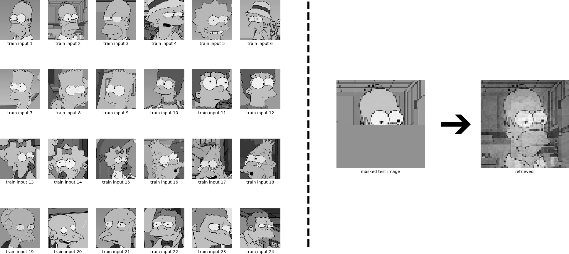
For 24 stored patterns:
For clarity, let’s now again visualize what is going on here:

Conclusion
The aim of this blog post has been to describe relations between the recently introduced Performer models and properties of continuous classical and continuous modern Hopfield Networks:
- Performers resemble classical Hopfield Networks.
- Sparseness increases memory capacity.
- Performer normalization relates to the activation function of continuous Hopfield Networks.